The Self Calibration Method for Multiple Systems at the CHARA Array

ScholarWorks @ Georgia State University

ScholarWorks @ Georgia State University

Mathematics Theses Department of Mathematics and Statistics

Spring 4-27-2011

A Review of Cross Validation and Adaptive Model Selection

A Review of Cross Validation and Adaptive Model Selection

Ali R. Syed

Georgia State University

Follow this and additional works at: https://scholarworks.gsu.edu/math_theses

Part of the Mathematics Commons

Recommended Citation Recommended Citation

Syed, Ali R., "A Review of Cross Validation and Adaptive Model Selection." Thesis, Georgia State University, 2011.

https://scholarworks.gsu.edu/math_theses/99

by

ALI RAZA SYED

Under the Direction of Yixin Fang

ABSTRACT

We perform a review of model selection procedures, in particular various cross validation

pro-cedures and adaptive model selection. We cover important results for these propro-cedures and explore

the connections between different procedures and information criteria.

by

ALI RAZA SYED

A Thesis Submitted in Partial Fulfillment of the Requirements for the Degree of

Master of Science

in the College of Arts and Sciences

Georgia State University

Copyright by Ali Raza Syed

by

ALI RAZA SYED

Committee Chair: Yixin Fang

Committee: Yichuan Zhao

Jiawei Liu

Electronic Version Approved:

Office of Graduate Studies

College of Arts and Sciences

Georgia State University

DEDICATION

ACKNOWLEDGEMENTS

I am grateful to the Department of Mathematics and Statistics at Georgia State University for

the instruction I received during my Masters in Statistics. In particular, I thank Dr. Fang for some great

conversations concerning research topics and for inspiring me to delve further into some exciting areas I

may otherwise have never learned about. I also wish to thank the excellent teachers I have had in many

classes which includes, but is not limited to, Dr. Zhao, Dr. Han, Dr. Qin and Dr. Zhang. I entered the

pro-gram knowing very little about discipline of Statistics, and while I have much further to go before

TABLE OF CONTENTS

ACKNOWLEDGEMENTS ... v

LIST OF FIGURES ... viii

1 INTRODUCTION ... 1

1.1 The “Best” Model ... 1

1.2 Information Criteria ... 2

1.3 Adaptive Model Selection ... 3

1.4 Cross Validation ... 4

1.5 Overview of the Remainder ... 4

2 CROSS VALIDATION ... 6

2.1 Leave-One-Out Cross Validation ... 6

2.1.1 Leaving-one-out lemma ... 7

2.2 Generalized Cross Validation ... 8

2.2.1 Asymptotic Equivalence with AIC ... 9

2.2.2 Further Note on the AIC/LOO Connection ... 9

2.3 Leave-K-Out Cross Validation ... 10

2.4 K-Fold Cross Validation ... 11

2.5 Choosing a Cross Validation Method ... 12

3 ADAPTIVE MODEL SELECTION ... 13

3.2 Generalized Degrees of Freedom ... 14

3.3 Adaptive Model Selection Procedure ... 15

3.4 GCV Analog... 16

4 SIMULATION ... 17

4.1 Adaptive Model Selection ... 17

5 REFERENCES ... 20

6 APPENDICES ... 22

LIST OF FIGURES

Figure 4.1 MSE from simulations for 3 procedures ... 18

1 INTRODUCTION

Model selection in statistics is the procedure of selecting the “best” model among a set of

com-peting models. A model is judged to be “best” according to some criteria. A common and prevailing

approach is to balance goodness of fit with parsimony. Goodness of fit determines how well the model

describes the data. However, increasingly complex models, with increasing number of parameters, are

bound to provide better fits at the expense of fitting to the noise as well as the data. This leads to the

phenomenon of over-fitting: the model describes the trained data well, but fails to take into generalize

to new data. The principle of parsimony, related to Occam’s razor, advocates choosing simpler models,

with fewer parameters. By balancing model complexity with goodness of fit, we can develop models

with lower generalization error.

Cross validation is a method of measuring generalization error through the use of holdout data.

There are many cross validation techniques and one of the most common is leave-one-out cross

valida-tion (LOO). Adaptive model selecvalida-tion uses a generalizavalida-tion of penalized criteria for model selecvalida-tion

where the penalty is based on the data (X. Shen & Ye, 2002). The adaptive selection procedure has the

advantage of performing well across a number of different modeling procedures.

This thesis reviews selected important theory concerning these model selection procedures. In

this chapter, we continue with a brief sketch of important concepts. In the remaining chapters, we

re-view cross validation procedures and adaptive model selection in greater detail and the connections

be-tween various procedures and information criteria.

1.1 The “Best” Model

Faced with competing models, we must first consider criteria for choosing between competing

much philosophy of science surrounding this topic. In a statistical modeling framework, we are usually

concerned with one of two goals for model selection: model estimation or model identification. Model

identification has the goal of minimizing a loss function and the desire here is for a statistically efficient

model selection procedure. This is commonly the goal in predictive modeling. Model identification has

the goal of finding the smallest optimal model describing the data, or the “true” model in this sense, and

the desire here is for a statistically consistent model selection procedure. This is commonly the goal in

descriptive modeling where we seek to explain a natural or social phenomenon.

1.2 Information Criteria

Given that the true model is unknown to us, we try to quantify the loss of information from the

approximate model in consideration M over the available dataD. We seek to minimize an information

criterion

GIC

with the general formulation:

2 (

, )

|

|

GIC

= −

L M D

+

λ

M

_.

(

)

L M

is the log-likelihood of the data D given the model M and

λ

is factor controlling the

penalty exacted for the model’s complexity. The first term measures the goodness of fit (GOF) while the

second term controls for model complexity. In fitting the model, the likelihood of D given M is found

by using the maximum likelihood estimates of the model parameters in M and represents an averaged

maximized log-likelihood rather than the expected maximized log-likelihood. Thus, the second term

may also be interpreted as a bias estimation to correct for this fact (Sima, 2006). This combination of

trading between goodness of fit and complexity may also be seen as the trade-off between bias and

va-riance.

In a classical least squares model, ignoring additive constants and multiplying through by

σ

2

re-sults in an equivalent formulation for minimization:

2

|

|

RSS

is the residual sum of squares. There are a number information criteria, derived from

dif-ferent theoretical considerations, each using a difdif-ferent penalty factor

λ

. Two common criteria are the

AIC (Akaike Information Criterion) and BIC (Bayesian Information Criterion). In AIC,

λ

=

2

and in BIC,

log

n

λ

=

where n is the number of observations in our data. AIC arises from information theoretic

foundations by considering the expected Kullback-Liebler divergence between the true and

approx-imated models. BIC arises from Bayesian decision-theoretic foundations using the Bayes factor. The BIC

exacts a heavier penalty than AIC for more complex models. Very generally, the AIC is preferred for

model estimation in predictive modeling due to its asymptotic efficiency property, while the BIC is

pre-ferred for model identification in descriptive modeling due to its asymptotic consistency property

(Clarke, Fokoue, & H. H. Zhang, 2009).

1.3 Adaptive Model Selection

We consider adaptive model selection (X. Shen & Ye, 2002) because of its connection to

infor-mation criteria and important properties in controlling for model complexity. In adaptive model

selec-tion, the

λ

factor is a data-adaptive penalty derived using the generalized degrees of freedom for a

giv-en modeling procedure. Ye defines a model selection procedure as having two parts: selection followed

by fitting. Consider the variable selection problem in linear regression, where a set of variables must be

chosen from a pool of candidate variables. The selection process results in the subset of variables in

consideration, while the fitting process determines the goodness of fit for the given subset. Applying

the traditional information criteria, such as AIC or BIC, does not correct for the bias induced by the

vari-able selection process. By considering the modeling procedure in totality, the adaptive model selection

adjusts for the selection bias. Specifically, it is found that the optimal

λ

ˆ

is obtained by minimizing:

2 ( )

RSS

+

G

λ

_.

( )

1.4 Cross Validation

In addition to Information Criteria, cross validation is another popular set of techniques used in

model selection. The general procedure is to partition the data into subsets for training and testing.

Training is the process of fitting a model while testing is the process of validating the fitted model

through measuring the prediction error. The training and test sets are disjoint so the testing data for

model evaluation are not used in model fitting. Cross validation is used across a range of areas such as

parameter selection, density estimation, classification and stopping criteria in neural networks. Cross

validation is not an information criterion in the sense that it does not penalize a goodness of fit

meas-ure. However, there exist asymptotic equivalences between cross-validation techniques and some

in-formation criteria.

1.5 Overview of the Remainder

There are a variety of model selection procedures in the statistical literature and the foregoing

highlights some of the commonly used procedures. In the subsequent chapters, we review cross

valida-tion and adaptive model selecvalida-tion in greater detail. Informavalida-tion criteria are not considered in great

depth since these are covered in various statistics classes; the introduction above serves as a summary

for exploring connections between information criteria and the procedures we will review. In general,

we will examine the procedures and their properties in the context of linear models of the form:

'

Y

=

X

β

+

ε

.

It is understood that Y is a

n

×

1

vector for n observations, X is a n×pvector of observed

values for p variables,

ε

is a

n

×

1

vector with ε

∼

N

(

0,

σ

2I

)

and

β

is an unknown

p

×

1

vector of

coefficients to be estimated. In some cases, we denote

f

as the function to be estimated through the

va-riables and estimate an optimal modelMˆ_k with cardinality

|

M

|

=

k

. However, many of the selection

2 CROSS VALIDATION

Suppose a dataset

D

=

{( ,

x

_i

y

_i

),

i

=

1,

…

, }

n

and we wish to assess a regression model M to

arrive at a corresponding set of predicted values

y

ˆ ,

_i

i

=

1,

…

,

n

. We can partition the dataset D into

two sets:

D

=

D

₁

∪

D

₂, with

k

data in

D

₁ and

n k

−

data in

D

₂. We fit the model M using the

data-set

D

₂; this is also known as training the model and

D

₂ as the training set. We then use the trained

model M to obtain predictions for observations

1

ˆ

D

Y

given 1 D

X ; this is also known as testing the model

and

D

₁ as the test set. There are n k

 

 

 

possible partitions of the data and this process can be repeated

multiple times. The CV estimate of error is the average prediction error over test sets used and this is

estimation of the average generalization error from applying our fitted function to an independent test

sample (Clarke, Fokoue, & H. H. Zhang, 2009).

2.1 Leave-One-Out Cross Validation

When

k

=

1

is used in the above formulation, the process is called leave-one-out cross

valida-tion (LOOCV), which we review in some depth because of a number of important connecvalida-tions. In this

case, our test set always has cardinality 1, and each of the

i

=

1,

…

,

n

possible partitions are used to train

and test the model. For eachi, let

ˆ

i

y

− denote the predicted value of left-out observation. The

leave-one-out cross validation estimate of error is:

2 1 1 ( ) n i i i i

LOOCV y y

n − = − =

∑

.

The general idea of leave-one-out cross validation appears to have been known for a while,

ex-tracts all information from given data without further justification. In linear regression, the LOOCV

es-timate is known as the PRESS (prediction sum of squares) statistic.

2.1.1 Leaving-one-out lemma

For large samples, the LOOCV estimate seems to have a heavy computational cost requiring n

model fits. An interesting result obviates this requirement for certain modeling procedures which are

linear in the observations, with

Y

ˆ

=

H

Y

, H _{being the influence or hat matrix, and requires only one fit}

over the entire datasetD. In this case, let

h

_ii denote the diagonal entries ofH, then the statistic is

cal-culated as: 2

1

1

ˆ

1

i i ii

n

LOOCV

n

i

y

y

h

=

=

−

−





∑ 







_.

This result holds for linear regression models and cubic smoothing splines, among other procedures,

which satisfy the leaving-one-out lemma (Wahba, 1990) stated below.

Denote ɶyi =( ,y₁ …,y_i−1,yˆ_i−i,y_i+1,…,y_n) as the consequence of replacing ith component of

Y with

ɵ

y

_i−i, and denote f−ias the estimate of our fitting function

f

given dataɶyi. The

leaving-one-lemma states (Wahba, 1990):

i

_{( )}

i

_{( ),}

_1,

_,

i i

f

−

x

=

f

−

x

i

=

…

n

.

The geometric interpretation here is that adding a new point exactly on the surface of f−i

leaves the fitted regression unaltered in the given system (Clarke, Fokoue, & H. H. Zhang, 2009). Since

our system is linear in the observations with

H

=

H

( )

X

, we have:

ɵ

ɵ

1

ˆ ( )

( )

(

)

n n _{i i}

i

i i ij j ij j ii i ii i i

j j i

f x

f

−

x

h y

h y

h y

−

h y

y

−

Applying the leave-one-out lemma, we obtain:

ɵ

ɵ

ɵ

ˆ_{( ) ( )} ˆ_{( ) ( ) ( )}

1

i i

i

i i i i ii i i

i i

ii i

i i

f x f x f x f x h y y

y y h y y − − − − − = − = − − ⇒ _{= −} − _.

Using this expression in the original LOOCV equation leads to the revised equation. Since the

revised form requires only one model fit over the entire data, the computational savings are

considera-ble. We will exploit this connection further when we consider an analogous criterion for adaptive model

selection.

2.2 Generalized Cross Validation

The generalized cross validation criterion (GCV) (Wahba, 1990) is an approximation to the

LOOCV and follows from noting that

1 tr( ) n ii i h = =

∑

H _{followed by the approximation:}

1

_{( )}

ii

h

tr

n

≈

H

_{. This}

is generally applicable when fitting linear methods with quadratic loss function and is a good

approxima-tion provided

h i

_ii

,

= …

1,

,

n

are not very different (Wahba, 1990). The generalized cross validation

sta-tistic becomes: 2 1 ˆ 1 1

1 ( )

n i i i y y GCV n _tr n =    ₋  =    ₋   

∑

H .

If the leaving-one-out lemma holds, then the generalized cross validation criterion may provide

further computational savings since it requires finding the trace rather than the individual diagonal

2.2.1 Asymptotic Equivalence with AIC

The generalized cross validation statistic as an approximation to the leave-one-out statistic is

al-so useful for examining analytic properties. Here we use the approximation to show the asymptotic

equivalence of leave-one-out cross validation to the AIC (Clarke, Fokoue, & H. H. Zhang, 2009). Consider

variable selection in a linear regression mode M where we evaluate a fixed subset of variables of size

|

M

|

. Since

tr

( ) |

H

=

M

|

_{in linear regression, and noting that} 2

ˆ

( ) ( i i)

RSS M =

∑

y −y , we have:

2

1

(

)

(

)

(1 |

| / )

RSS M

GCV M

n

M

n

=

−

_.

For large n, when

|

M

| /

n

is small, we can apply a Taylor expansion,

(1 |

−

M

| / )

n

−2

≈

1 2 |

+

M

| /

n

to

arrive at:

(

)

(

) |

|

(

)

RSS M

2

RSS M

M

GCV M

n

n

n

≈

+

.

Further note that asn→ ∞,

RSS M

(

) /

n

→

σ

2and rewriting the above expression as:

2

(

)

|

|

(

)

RSS M

2

M

GCV M

n

σ

n

≈

+

.

We see that minimizing the GCV is equivalent to minimizing AIC. Note that the connection to Mallow’s

p

C in linear regression is more apparent here and, in fact, AIC is equivalent to Mallow’s C_pin linear

regression. Another point we can note is that although the estimate of the variance in linear regression,

and consequently Mallow’s C_pis based on

(

n

−

p

)

degrees of freedom, our substitution above is valid

asymptotically.

2.2.2 Further Note on the AIC/LOO Connection

The above is not a real proof of equivalence but simply suggestive of the connection between

and is not limited to linear models. Consequently, the log-likelihood of the data can be approximated

through the likelihood based LOOCV, or comparisons can be made based on LOOCV error statistic. This

becomes useful when faced with models where the likelihood is analytically difficult to compute.

Stone’s proof also holds for the Takeuchi Information Criterion (TIC), a general form of the AIC, which

involves computing the trace of a product involving the Fisher information matrix and the score function

(Lee, 2007). This trace reduces to the number of parameters in the case of exponential family of

distri-butions, but not generally. The asymptotic connection to the LOOCV may then be useful as an

alterna-tive to analytically difficult computations. However, the LOOCV carries its own computational cost and

can be an expensive procedure when the GCV approximation does not hold.

We can also try to gain an intuitive understanding of the asymptotic equivalence by noting that

the AIC minimizes the KL divergence between the approximate model and the true model. The KL

diver-gence is not a distance measure between distributions, but really a measure of the information loss

when the approximate model is used to model the ground reality. Leave-one-out cross validation uses a

maximal amount of data for training to make a prediction for one observation. That is,

n

−

1

observa-tions as stand-ins for the approximate model relative to the single observation representing “reality”.

We can think of this as learning the maximal amount of information that can be gained from the data in

estimating loss. Given independent and identically distributed observations, performing this over n

possible validation sets leads to an asymptotically unbiased estimate.

The LOOCV method shares similar statistical properties with AIC: it provides asymptotically

un-biased result for the true prediction error by trading off with variance.

2.3 Leave-K-Out Cross Validation

In the formulation at the start of this chapter, leave-k-out cross validation (LKOCV) is the general

computational expense due to the n k

   

 possible partitions that must be left-out and is rarely used in

practice (Sylvain & Celisse, 2010).

2.4 K-Fold Cross Validation

An alternative procedure is K-fold cross validation and this procedure was motivated by

compu-tational expense of the leave-one-out procedure (Geisser, 1975). The K-fold procedure is attractive

be-cause it balances computational cost with an increase in the estimation bias. In this procedure, the

da-taset Dis divided into K partitions of roughly equal size,

1 K k k D D =

=

_∪

, and each partition is termed a

“fold” of the dataset (thus there are Kfolds). The procedure may be understood as a

leave-one-fold-out procedure in analogy to the leave-one-leave-one-fold-out procedure. The model is trained on K−1 folds and the

Kth fold is used for testing (Clarke, Fokoue, & H. H. Zhang, 2009). This is repeated K times such that

each fold is used for testing exactly once. Setting

K

=

n

leads to leave-one-out cross validation.

Define an index function

κ

:{1,

…

, }

n

→

{1,

…

, }

K

as a scheme to randomly assign the ith

da-tum to a fold. Leaving out the

k

th fold for testing and fitting the model on the remaining

k

−

1

folds,

results in estimated model function fˆ−κ( )i . The cross validation statistic for prediction error is then

(Hastie, Tibshirani, & Friedman, 2001):

( )

1

2

1

ˆ )

( _i i

n

i

KCV y y

n κ − = =

∑

− .

The k-fold cross validation procedure is often applied to choose a model specific parameter.

Suppose that the models are indexed by parameter

λ

∈ Λ

with corresponding estimated model

func-tion fˆ_λ−κ( )i to be evaluated on the

k

th fold. The optimal

λ

ˆ

is chosen as (Hastie, Tibshirani, &

ɵ ( ) 2

1

1

ˆ

arg min ( ) arg min ( i i )

n

i

KCV y y

n

κ λ

λ λ

λ

λ

−

=

= =

∑

−

.

The final model is trained with the optimal parameter over the entire data, with the KCV statistic

re-ported as the cross validation prediction error. In general, the recommended values for K are 5 or 10 .

2.5 Choosing a Cross Validation Method

As with any model selection procedure, the bias and variance tradeoff influences the choice of

cross validation procedure. LOOCV is asymptotically unbiased as mentioned earlier. The choice of

train-ing set size influences our decision due to some important results in (Shao, 1993).

In general, choosing LOOCV or KCV with small size for the testing set results in an

overestima-tion of the variance, but relatively small bias. When the goal is model estimaoverestima-tion, and the sample has

low variance, a smaller bias is preferred. Thus the recommendation is to opt for LOOCV or KCV with

rel-atively small folds. The smallest bias is obtained when the training set size approaches the sample size,

i.e.

(

n k

−

)

→

n

as in LOOCV. The goal of model identification requires that a larger bias is induced since

consistency results require the training set size to be much smaller than the sample size (Sylvain &

Ce-lisse, 2010).

It is found that small variance in the CV statistic generally leads to optimal model selection

per-formance. In the cross validation cases covered here, the number of folds K is linked to the size of the

training set. In this case, it has been found that the variance of the CV statistic must be quantified

3 ADAPTIVE MODEL SELECTION

Minimizing information criteria are a popular choice of model selection. As reviewed above, for

model M these take the general form:

2 (

l M

)

λ

|

M

|

−

+

_.

(

)

l M

is the maximum log-likelihood of the model M ;

|

M

|

is the cardinality of the model; and

λ

is a

fixed penalty factor depending on the criterion. In linear regression, this is equivalent to minimizing the

form:

(

)

|

|

RSS M

+

λ

M

_.

(

)

RSS M

is the residual sum of squares from fitting the model.

One problem with such criteria is none of them perform uniformly well across a variety of

situa-tions. AIC, with penalty

λ

=

2

, performs well when the size of the true model is large but yields

sub-stantial bias when the model size is small. BIC, with a heavier penalty

λ

=

log( )

n

, performs well when

the size of the true model is small, but yields substantial selection bias with large models (B. Zhang,

2010). The motivation for an adaptive model selection procedure (X. Shen & Ye, 2002) is to produce a

data-adaptive penalty that reduces the selection bias across the range of situations. The basis for the

data-adaptive penalty is the generalized degrees of freedom (Ye, 1998).

3.1 Degrees of Freedom

In linear regression, the degrees of freedom are best understood through geometric

considera-tion and may be defined as the dimension of the estimaconsidera-tion subspace (Walker, 1940). In the simplest

case of a linear system with p independent variables per observation, we seek the least squares

projec-tion of the n-dimensional observation vector Y in a p-dimensional estimation subspace. There are

the number of independent parameters in our system. The system is linear in the observations through

the projection matrix

H

=

H

( )

X

, also known as the hat matrix. Increasing the dimension of our

esti-mation subspace reduces the least squares distance between Y and its projection

Y

=

H

Y

_{at the cost}

of introducing a more complex structure for our estimation subspace. Thus the degrees of freedom are

a measure of model complexity and this is the term penalized by the various information criteria.

A similar notion extends to systems outside the least squares class as long as they are linear in

the observations, i.e. with

Y

=

H

Y

_{. In such cases, a variety of definitions exist for different systems as}

the effective degrees of freedom, usually the trace of some function

d

of the hat matrix:

tr d H

( ( ))

. In

linear regression, the degrees of freedom are equivalent to

ɵ

( ) i

ii

i

y

tr H h

y

∂

= =

∂

∑

∑

, “the sum of the

sensitivities of the fitted values with respect to the observed response values” (Ye, 1998).

3.2 Generalized Degrees of Freedom

The generalized degrees of freedom (GDF) is a generalization of the concepts of degrees of

free-dom mentioned above. In addition, the observation, given above, of degrees of freefree-dom as the sum of

sensitivities of fitted to response values motivates Ye’s definition of GDF in linear models (Ye, 1998):

0 1 1 2 2 1 1

(

)

( )

E

( )

(

)

lim E

E

( )(

)

cov(

( ),

)

n n

i i

i i

i i i

n n

i i i i i i

i i

GDF M

y

y

δ

µ

δ

µ

µ

µ

δ

µ

µ

µ

µ

σ

σ

→ = = = =



₊

₋



∂

=

=





∂



_



_

−

−

=

=

∑

∑

∑

∑

Y

e

Y

Y

Y

Y

.

The GDF is defined as the “sum of average sensitivities of the fitted value

µ

ˆ ( )

_i

Y

_{to a small}

change in

y

_i”. It is a measure of the flexibility of the modeling procedure $M$. In the same that the

overfit, the GDF enables us to consider the complexity of the modeling procedure and its tendency to

overfit. In this way, the GDF depend on the “true” model and modeling procedure.

The notion of GDF was extended to a general class of modeling procedures using an optimal loss

formulation which is consistent with the GDF definition given above (Xiaotong Shen & Huang, 2006).

3.3 Adaptive Model Selection Procedure

The adaptive selection criterion takes the form:

ɵ

( ) | |

RSS M +

λ

M _.

ˆ

λ

is the data-adaptive penalty in the sense that it grows when the size of the true model is small, and

shrinks when the size of the true model is large. It also adapts in the sense of approximating optimal

performance over the class of information criteria. It is found that the optimal penalty is obtained by

when the following expression is minimized, which coincides with the GDF as previously stated:

ɵ

_{arg min}

_RSS

_{2 ( ),}

_G

_{(0, )}

λ

λ

=

+

λ λ

∈

∞

.

For variable selection in linear models over a class of models

M

( )

λ

, the procedure is as follows.

ɵ

λ

is determined by minimizing the above expression. For each fixed

λ

, we determine the least squares

fit for

M

( )

λ

. G( )

λ

is found by using a Monte Carlo regression procedure (X. Shen & Ye, 2002):

• Sample

δ

_j from n-dimensional

N

(0,

τ

2

I

)

where

τ

=

0.5

σ

.

• Compute the

µ

ˆ_{Mˆ ( )λ} (y

+

δ

_j), j

=

1,…,T .

• Compute the regression slope ˆ_{ˆ ( )}( _j) ɵi _ji, 1, ,

M λ y a j T

µ

+

δ

= +

λ δ

= …

. o 1 ˆ ( ) n i i

G

λ

λ

=

=

∑

3.4 GCV Analog

Ye defines a GDF analog (Ye, 1998) to the GCV criterion for model M as

2

(

)

(

)

(

(

))

RSS M

GCV M

n GDF M

=

−

_.

Given the GCV derivation from the previous chapter, we show how this is derived. Recall that after

ap-plying the leaving-one-out lemma is satisfied, we have:

ɵ

ɵ ɵ

ɵ

ɵ

ˆ_{( )} i_{( )} ˆ_{( )} i_{( ) (} i₎

i i i i ii i i

i

i i i i

ii i

i i

i i

f x f x f x f x h y y

y y y

h y y y y

µ

− − − − −

−

=

−

=

−

−

∆

∂

⇒

₌

₌

_≈

∆

∂

−

_.

Using this in the expression for the LOOCV, with the approximation

(

)

i

ii

i

h

GDF M

y

µ

∂

=

=

∂

∑

∑

, we

arrive at:

2

(

)

(

)

(1

(

) / )

RSS M

GCV M

GDF M

n

=

−

_.

4 SIMULATION

4.1 Adaptive Model Selection

We reproduce one of the simulations performed by Ye to better understand the adaptive model

selection procedure through implementation. The code in the R language is provided in the appendix.

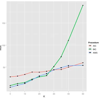
The chart below shows the MSE values for different model selection procedures against the

number of true variables in the model. Our results are comparable to those of the paper. Note that in

the legend, “AMS” refers to “Adaptive Model Selection” and K refers to the number of non-zero

[image:28.612.122.500.78.453.2]

Figure 4.1 MSE from simulations for 3 procedures K

M

S

E

50 100 150

0 10 20 30 40 50

Procedure

AIC

BIC

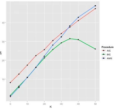
The next figure shows the average number of variables selected by the different procedures for

[image:29.612.87.474.159.535.2]

given number of non-zero variables in the true model.

Figure 4.2 Number of variables selected by the different procedures K

p

0

10 20 30 40

0 10 20 30 40 50

Procedure

AIC

BIC

5 REFERENCES

Clarke, B., Fokoue, E., & Zhang, H. H. (2009). Principles and Theory for Data Mining and Ma-chine Learning (Springer Series in Statistics) (p. 798). Springer. Retrieved from

http://www.amazon.com/Principles-Machine-Learning-Springer-Statistics/dp/0387981349.

Geisser, S. (1975). The Predictive Sample Reuse Method with Applications. Journal of the American Statistical Association, 70(350), 320-328. Retrieved from

http://www.jstor.org/stable/2285815.

Hastie, T., Tibshirani, R., & Friedman, J. (2001). The Elements of Statistical Learning. Book (Vol. 2, p. 764). Springer. doi: 10.1007/978-0-387-84858-7.

Lee, H. (2007). Cross-validation for model selection. Retrieved from

http://groundtruth.info/AstroStat/slog/2007/cross-validation-for-model-selection/.

Shao, J. (1993). Linear Model Selection by Cross-Validation. Journal of the American Statistical Association, 88(422), 486. doi: 10.2307/2290328.

Shen, X., & Ye, J. (2002). Adaptive model selection. Journal of the American Statistical Associ-ation, 97(457), 210–221. ASA. Retrieved March 18, 2011, from

http://pubs.amstat.org/doi/pdf/10.1198/016214502753479356.

Shen, Xiaotong, & Huang, H.-C. (2006). Optimal Model Assessment, Selection, and Combina-tion. Journal of the American Statistical Association, 101(474), 554-568. doi:

10.1198/016214505000001078.

Sima, D. M. (2006). Regularization Techniques in Model Fitting and Parameter Estimation. Re-trieved from ftp://ftp.esat.kuleuven.ac.be/pub/SISTA/dsima/reports/thesisDianaSima.html.

Stone, M. (1977). An asymptotic equivalence of choice of model by cross-validation and Akaike

ʼ

s criterion. Journal of the Royal Statistical Society. Series B (Methodological), 39(1), 44–47. JSTOR. Retrieved March 18, 2011, from

http://www.jstor.org/stable/2984877.

Sylvain, A., & Celisse, A. (2010). A survey of cross-validation procedures for model selection. Statistics Surveys, 4, 40-79. doi: 10.1214/09-SS054.

Wahba, G. (1990). Spline Models for Observational Data. Society for industrial and applied ma-thematics.

Ye, J. (1998). On Measuring and Correcting the Effects of Data Mining and Model Selection. Journal of the American Statistical Association, 93(441), 120- 131. American Statistical Association. Retrieved March 18, 2011, from

http://www.questia.com/PM.qst?a=o&se=gglsc&d=5002287558.

6 APPENDICES

Appendix A

rm(list=ls())

if (.Platform$OS.type == 'unix') { require(doMC)

registerDoMC() }

else if (.Platform$OS.type == 'windows') { require(doSNOW)

.clusters <- makeCluster(2, type='SOCK') registerDoSNOW(.clusters) } require(MASS) require(DAAG) require(leaps) require(foreach)

cat('getDoParWorkers', getDoParWorkers(), '\n') cat('--- Start script:', date(), '\n')

start <- Sys.time()

#--- # utils

#---

# return px1 B such that theoretical R.sq = r.sq # p must be multiple of 5

# k: num non-zero coefs per 5-vector subset find.beta <- function(x, n, p, k, r.sq) {

k.max <- 10 if (k == 0) {

B <- rep(0, p) } else {

bk <- rep(c(1, 0), c(k, k.max-k)) b <- rep(bk, p/k.max)

xx <- t(x) %*% x

B.k.sq <- (r.sq * n) / ( (1 - r.sq) * (t(b) %*% xx %*% b) ) B <- sqrt(B.k.sq[1]) * b

}

array(B, dim=c(p, 1), dimnames=list(paste('b', 1:p, sep=''))) }

gen.x <- function(n, p, x.Sigma) { require(mvtnorm)

x <- rmvnorm(n, mean=rep(0, p), sigma=x.Sigma) colnames(x) <- paste('x', 1:p, sep='') x

gen.vars <- function(n, p, k, r.sq, x.Sigma, y.sigma) { x <- gen.x(n, p, x.Sigma)

b <- find.beta(x, n, p, k, r.sq) mu <- x %*% b

y <- mu + array(rnorm(n, mean=0, sd=y.sigma), dim=c(n, 1)) colnames(y) <- 'y'

fo.full <- formula(paste('y~0+', paste('x', 1:p, sep='', collapse='+')))

list(y=y, x=x, b=b, mu=mu, fo.full=fo.full) }

fit.step <- function(lambda, data) { fit.lower <- lm(y ~ 0, data=data)

fit <- stepAIC(fit.lower, scope=form.upper, k=lambda, direc-tion='forward', trace=FALSE)

fit }

adaptive <- function(y, x, p) {

data <- as.data.frame(cbind(y, x))

pert <- replicate(pert.T, rnorm(n, mean=0, sd=pert.tau)) pert.y <- pert + matrix(y, nrow=n, ncol=pert.T, byrow=FALSE)

pert.subs <- foreach(j=1:pert.T, .packages=c('leaps')) %dopar% { subs <- regsubsets(x, pert.y[ , j], method='forward', nvmax=p,

intercept=FALSE, really.big=TRUE) summary(subs)

}

cache.g <- cache.G <- cache.lam <- c() f.g <- function(lambda) {

lam <- round(lambda, 2)

pkg <- c('leaps')

expt <- c('pert.subs', 'x', 'p')

pert.mu <- foreach(j=1:pert.T, .combine=cbind, .export=expt, .packages=pkg) %dopar% {

ye.ic <- pert.subs[[j]]$rss + lam * (1:p) model.idx <- which.min(ye.ic)

coef.idx <- pert.subs[[j]]$which[model.idx, ]

b <- rep(0, p)

b[coef.idx] <- coef(pert.subs[[j]]$obj, model.idx) bb <- matrix(b, nrow=50, ncol=1)

fit <- x %*% b fit

}

g0 <- foreach(i=1:n, .combine=sum, .export=c('pert')) %dopar% { fit.sens <- lm(pert.mu[i, ] ~ pert[i, ])

return( g0 ) }

f.G <- function(lambda) { lam <- round(lambda, 2) if (any(cache.lam == lam)) {

return( cache.G[which(cache.lam == lam)] ) }

g0 <- f.g(lam)

fit <- fit.step(lam, data) G <- sum( resid(fit)^2 ) + g0

cache.lam <<- c(cache.lam, lam) cache.g <<- c(cache.g, g0) cache.G <<- c(cache.G, G)

return( G ) }

res <- optimize(f.G, interval=c(0, 20)) lambda.hat <- round(res$minimum, 2)

g0 <- cache.g[which(cache.lam == lambda.hat)] return( list(lam=lambda.hat, gdf=g0/2) ) }

#--- # constants

#--- p <- 50

n <- 200

ks <- c(0, 3, 7, 10)

#ks <- c(1, 2, 4, 5, 6, 8, 9) nsims <- 50

r.sq <- 0.75 y.sigma <- 1 x.Sigma <- diag(p)

pert.T <- n + 20 pert.tau <- 0.5

# full model as upper bound for stepwise selection

form.upper <- formula(paste('~0+', paste('x', 1:p, sep='', collapse='+')))

cat('p:', p, 'n:', n, 'nsims:', nsims, 'pert.T:', pert.T, '\n')

k.results <- list() for (k in ks) {

coln <- c('mse.aic', 'mse.bic', 'mse.lam', 'p0.aic', 'p0.bic', 'p0.lam', 'gdf', 'lambda', 'k', 'p', 'n')

sim.results <- array(NA, dim=c(nsims, 11), dimnames=list(sim=1:nsims, coln))

for (isim in 1:nsims) {

cat(' isim', isim, date(), '\n') s2 <- Sys.time()

vars <- gen.vars(n, p, k, r.sq, x.Sigma, y.sigma)

res <- adaptive(vars$y, vars$x, p)

cat(' lambda:', res$lam, ', gdf:', res$gdf, '\n')

data <- as.data.frame(cbind(vars$y, vars$x)) pkg <- c('MASS')

penalties <- c(aic=2, bic=log(n), lam=res$lam)

res.fits <- foreach(pen=penalties, .combine=cbind, .packages=pkg) %dopar% {

fit <- fit.step(pen, data) p0 <- length(coef(fit))

mse <- sum( (vars$mu - fitted(fit))^2 ) c(mse=mse, p0=p0)

}

colnames(res.fits) <- names(res.fits) print(res.fits)

sim.results[isim, ] <- c(res.fits[1, ], res.fits[2, ], gdf=res$gdf, lambda=res$lam,

k=k, p=p, n=n) fname <- paste('sim-k', k, 's', nsims, 'Rd', sep='.') save(sim.results, file=fname)

f2 <- Sys.time()

runt <- as.numeric(difftime(f2, s2, units='secs'))

cat(' time:', runt, 'secs,', round(runt/60, 1), 'mins', round(runt/60/60, 2), 'hours', '\n')

}

k.results[[as.character(k)]] <- sim.results

fname <- paste('k-k', k, 'ns', nsims, 'Rd', sep='.') save(k.results, file=fname)

f1 <- Sys.time()

runt <- as.numeric(difftime(f1, s1, units='secs'))

cat(' time:', runt, 'secs,', round(runt/60, 1), 'mins', round(runt/60/60, 2), 'hours', '\n')

}

cat('--- End script:', date(), '\n') end <- Sys.time()

cat('Run time:', runtime, 'secs,', round(runtime/60, 1), 'mins', round(runtime/60/60, 2), 'hours', '\n')

if (.Platform$OS.type == 'windows') { stopCluster(.clusters)