www.copernicus.org/EGU/hess/hess/9/243/ SRef-ID: 1607-7938/hess/2005-9-243 European Geosciences Union
Earth System
Sciences
Rainfall-runoff modelling in a catchment with a complex
groundwater flow system: application of the Representative
Elementary Watershed (REW) approach
G. P. Zhang and H. H. G. Savenije
Water Resources Section, Faculty of Civil Engineering and Applied Geosciences, Delft University of Technology, Stevinweg 1, P.O. Box 5048, 2600 GA Delft, The Netherlands
Received: 7 March 2005 – Published in Hydrology and Earth System Sciences Discussions: 12 May 2005 Revised: 11 August 2005 – Accepted: 2 September 2005 – Published: 21 September 2005
Abstract. Based on the Representative Elementary Water-shed (REW) approach, the modelling tool REWASH (Rep-resentative Elementary WAterShed Hydrology) has been veloped and applied to the Geer river basin. REWASH is de-terministic, semi-distributed, physically based and can be di-rectly applied to the watershed scale. In applying REWASH, the river basin is divided into a number of sub-watersheds, so called REWs, according to the Strahler order of the river net-work. REWASH describes the dominant hydrological pro-cesses, i.e. subsurface flow in the unsaturated and saturated domains, and overland flow by the saturation-excess and infiltration-excess mechanisms. The coupling of surface and subsurface flow processes in the numerical model is realised by simultaneous computation of flux exchanges between sur-face and subsursur-face domains for each REW. REWASH is a parsimonious tool for modelling watershed hydrological re-sponse. However, it can be modified to include more com-ponents to simulate specific processes when applied to a spe-cific river basin where such processes are observed or con-sidered to be dominant. In this study, we have added a new component to simulate interception using a simple paramet-ric approach. Interception plays an important role in the wa-ter balance of a wawa-tershed although it is often disregarded. In addition, a refinement for the transpiration in the unsat-urated zone has been made. Finally, an improved approach for simulating saturation overland flow by relating the vari-able source area to both the topography and the groundwater level is presented. The model has been calibrated and veri-fied using a 4-year data set, which has been split into two for calibration and validation. The model performance has been assessed by multi-criteria evaluation. This work represents
Correspondence to: G. P. Zhang
a complete application of the REW approach to watershed rainfall-runoff modelling in a real watershed. The results demonstrate that the REW approach provides an alternative blueprint for physically based hydrological modelling.
1 Introduction
Hydrological models are important and necessary tools for water and environmental resources management. Demands from society on the predictive capabilities of such models are becoming higher and higher, leading to the need of en-hancing existing models and even of developing new the-ories. Existing hydrological models can be classified into three types, namely, 1) empirical models (black-box mod-els); 2) conceptual models; and 3) physically based models. To address the question of how land use change and climate change affect hydrological (e.g. floods) and environmental (e.g. water quality) functioning, the model needs to contain an adequate description of the dominant physical processes.
both the advantages and disadvantages of such models has arisen along with research and applications of those mod-els (see, e.g. Beven 1989, 1996a, b, 2002; Grayson et al., 1992b; Refsgaard et al., 1996; O’Connell and Todini, 1996). In general, such models are very data-intensive and time-consuming when applied in a fully distributed manner. In applications, the model scale is generally much larger than the scale of parameter measurements. Therefore, “effective” parameter values have to be adopted in model applications and thus calibration becomes inevitable for physically based models. This leads to the difficulty of parameter identifi-cation and the equifinality problem (Beven, 1993, 1996c; Savenije, 2001).
Conceptual models form by far the largest group of hydro-logical models that have been developed by the hydrologi-cal community and which are most often applied in opera-tional practice. Among those are SAC-SMA (Burnash et al., 1973; Burnash, 1995), HBV (Bergstr¨om and Forsman, 1973; Bergstr¨om, 1995), and LASCAM (Sivapalan et al., 1996). Most conceptual models are spatially lumped, neglecting the spatial variability of the state variables and parameters. To improve the potential for making use of spatially distributed data, some lumped conceptual models have been extended to be distributed or semi-distributed. Examples are the HBV-96 model (Lindstr¨om et al., 1997), TOPMODEL (Beven, 1995) and the ARNO model (Todini, 1996). Parameters of this type of models, however, either lack physical meaning or cannot be measured in the field. Parameter identifiability and equi-finality are the major concerns of such models.
In view of all these different types of modelling ap-proaches, one can notice that there is no commonly accepted general framework for describing the hydrological response directly applicable at watershed scale. To fill this gap, Reg-giani et al. (1998, 1999) made an attempt to derive a uni-fying framework for modelling watershed response, which has been named the Representative Elementary Watershed (REW) approach. This theory applies global balance laws of mass and momentum and yields a system of coupled non-linear ordinary differential equations at the REW scale, gov-erning flows between different sub-domains of a REW. To demonstrate the applicability of the REW approach, Reg-giani et al. (2000) investigated the long-term water balance of a single hypothetical REW using the equations in non-dimensional form. In that work, only hill-slope subsurface responses, i.e. flows in the unsaturated and saturated zones were considered. In succession, Reggiani et al. (2001) ap-plied the REW approach to a natural watershed but only fo-cusing on the response of the channel network. They pro-vided the theoretical development of the REW approach and demonstrated that the approach can provide a framework for an alternative blueprint for modelling watershed response (Beven, 2002; Reggiani and Schellekens, 2003).
Parallel to theory formulation, much work has been done to apply the REW approach towards the development of wa-tershed models. Zhang et al. (2003, 2004a, b, 2005a) and
Reggiani and Rientjes (2005) reported on advances of the research in this regard. However, as Beven (2002) pointed out while discussing about the REW approach, one should recognise that the balance equations alone are indeterminate, and additional functional relationships associated with the simplifying assumptions (i.e. the so called constitutive rela-tionships), for the fluxes within and between REWs, are cru-cial to the closure of the system. We would like to stress this issue as the closure problem. Lee et al. (2005) and Zehe et al. (2005) presented comprehensive discussions in this regard. One can understand that developing closure re-lations is in fact the way of parameterisation. Thus, proper closure relations are keys to a successful application of the approach. Zhang et al. (2005a) made a step towards a bet-ter model paramebet-terisation and showed encouraging results when applied to a temperate humid watershed. Meanwhile, it is obvious that an incomplete description of hydrological processes inevitably results in poor performance and leads to erroneous results. For instance, as pointed out by Savenije (2004, 2005), neglecting interception can introduce signifi-cant errors in other parameters. Moreover, previous research on the REW approach to modelling of actual catchments highlighted the need for significant improvements. There-fore, this paper reports on the current state of development of the REW approach within our research framework.
In this work, the numerical model REWASH has been de-veloped based on the original code dede-veloped by P. Reg-giani and reflected in the application presented in RegReg-giani and Rientjes (2005). REWASH includes the process of in-terception and a modified transpiration scheme for the un-saturated zone. The model has been applied to the Geer river basin and the model performance has been evaluated through calibration and verification procedures. Model calibration and verification have been carried out through a combination of manual and automatic calibration, and a split-sample test. Sensitivity analysis has been performed to examine model behaviour and identify the most important parameters. Mod-elling results show that the hydrographs can be well repro-duced and the model is able to simulate the watershed re-sponse at a large spatial scale in a lumped fashion while the parameters are kept physically meaningful. However, there is still considerable scope for improvement (e.g. Zhang et al., 2005b). It is realised that closure relations need to be watershed-specific, depending on the dominant mechanisms and data availability.
2 Mathematical representation of the hydrological pro-cesses
2.1 The concept of the REW approach
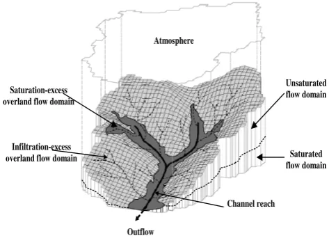
a watershed (hill-slopes and channels, Fig. 1). The discreti-sation is based on the analysis of the basin topography using the Strahler stream order system. The topographical bound-aries of REWs coincide with their surface water divides, thus REWs are naturally interconnected through the stream net-works as well as through the subsurface flow paths in terms of water flux exchanges. While determining the size of in-dividual REWs and their sub-domains, each REW is implic-itly defined in three dimensions and delimited externally by a prismatic mantle.
The volumetric entities of a REW contain flow domains commonly encountered or described within a watershed: 1) the unsaturated flow domain, 2) the saturated flow domain, 3) the saturation-excess overland flow domain, 4) the con-centrated overland flow domain (or the infiltration-excess overland flow domain), and 5) the river channel. Hydrologi-cal processes in these domains are characterised by different temporal scales. For instance, overland flow has a time scale of minutes to hours, while saturated groundwater flow has months to years (Bl¨oschl and Sivapalan, 1995).
In the REW approach, averaged balance equations of mass and momentum for each flow domain were derived (Reggiani et al., 1998, 1999), resulting in a set of non-linear ordinary differential equations (ODEs) which no longer contain any spatial information below the REW scale. In contrast to grid-based methods applied in most distributed model approaches (e.g. Abbott et al., 1986a, b), the REW approach uses the sub-watersheds (REWs) as “cells”, the basic discretisation units on which the ODEs are solved.
The general form of the ODEs reads: dφ
dt =
X
i
eφi+s (1)
whereφrepresents a generic thermodynamic property such as mass or momentum. eφi stands for a generic exchange term of φ ands is a grouped sink/source term for the do-main in question. This form can be extended to include terms for more complex flow phenomena, such as multi-phase flow and pollutants transport. As we know, the conservation equa-tion itself alone is not a closed system. The exchange term eφiis unknown and needs to be specified. This term has to be expressed in a form that relates the state variables to other re-solved variables. This comes to the problem of finding proper closure relations for the balance equations, as touched upon in the introduction. Closure relations for process descrip-tions at the catchment-scale, other than the point-scale or the REV (representative elementary volume) scale, are not read-ily available. However, after rigorous theoretical derivation, REW-scale equations for: Darcy’s law, Manning’s law, and the Saint-Venant equations have been obtained and employed in our model, which are valid for subsurface, overland and channel flow, respectively. The relations of these equations to the flux terms are summarised in Table 1 of the following section.
Outflow Atmosphere
Saturation-excess overland flow domain
Unsaturated flow domain
Channel reach
Saturated flow domain Infiltration-excess
[image:3.595.309.546.63.234.2]overland flow domain
Fig. 1. A 3-D view of the volume comprising a single REW
(modi-fied from Reggiani and Schellekens, 2003).
2.2 Description of the numerical model
In many hydrological models or model approaches, intercep-tion is neglected even though it is the first process in the chain of interlinked rainfall-runoff processes (Savenije, 2004). By ignoring this process, errors are introduced that propagate into the subsequent processes simulated (particularly into the soil moisture and groundwater flow process) and into the wa-ter balance regime in the different stores of a wawa-tershed, al-though sometimes they may not be detected by only looking at the single integral output: the simulated stream discharge. In the initial stage of the development and application of the REW approach, interception was not explicitly consid-ered. Bearing this in mind, we have added a component in this model using a simple parametric approach to account for the interception effect. In addition, in line with the work by Zhang et al. (2003, 2004a, b), a refinement for sub-grid vari-ability of soil properties in the soil column has been taken into account. Moreover, a new approach to determine the saturated overland area has been introduced. Based on these modifications, the water balance equations for the different flow domains and governing equations for the various flow processes are described below.
2.2.1 Water balance equations for flow domains
Average ground surface
Average bottom Average g.w. table
Datum
z
s
zr
ys
zsu
r
f
yu
γo Average river bed
ecu
eus
eua
Szone
Uzone Czone
Ozone
eso
esr River
eor eoa
esi
ectop
eotop
ertop era
[image:4.595.51.283.64.191.2]eca
Fig. 2. Schematised cross-sectional profile of a REW. Czone, Ozone, Uzone, Szone and River stand for the infiltration-excess overland flow domain, the saturation-excess overland flow domain, the unsaturated flow domain, the saturated flow domain and the River flow domain, respectively.ect op,ecu,ecaetc. are flux terms. yu,ys are stock variables, andzs,zr,zsurf andγoare average
ge-ometric quantities of the REW.
Infiltration-excess overland flow domain dSc
dt =ect op+eca+ecu+eco (2) where Sc (M) is the storage of the infiltration-excess over-land flow domain. The fluxes ect op (MT−1), eca (MT−1), ecu(MT−1) andeco(MT−1) are the rainfall on the surface of this zone, the evaporation from interception on this zone, the infiltration to the saturated zone and the transfer towards the saturation-excess flow domain, respectively. Since we are ap-plying this model approach to a humid temperate river basin where the saturation-excess flow is dominant, the infiltration-excess overland flow is negligible, thusecois kept zero. Saturation excess overland flow domain
dSo
dt =eot op+eoa+eos+eor+eoc (3) where So (M) is the storage of the saturation-excess over-land flow domain. The fluxeseot op(MT−1),eoa(MT−1),eos (MT−1),eor (MT−1) andeoc(MT−1) are the rainfall on the
surface of this zone, the evaporation from this zone, the ex-change between this zone and the saturated flow zone, the transfer to the river channel, and the exchange between this zone and the infiltration-excess flow zone, respectively. For the same reason stated above,eocis ignored.
Unsaturated subsurface flow domain dSu
dt =eua+euc+eus (4)
whereSu(M) is the storage of the unsaturated flow domain. The fluxeseua(MT−1),euc(MT−1), andeus(MT−1) are the transpiration, the infiltration and the percolation.
Saturated subsurface flow domain dSs
dt =esu+eso+esr+esi+esa (5) whereSs(M) is the storage of the saturated flow domain. The fluxes esu (MT−1) andeso (MT−1) are the counterparts of eus(MT−1) andeos(MT−1) in Eqs. (3) and (4), respectively; esr (MT−1),esi (MT−1) andesa (MT−1) are the exchange between the saturated zone and river channel, the exchange with the neighbouring REWs (if any) and the groundwater abstraction (if any).
River channel dSr
dt =ert op+era+ers+ero+erin+erout (6) where Sr (M) is the storage of the river channel segment within the REW under investigation. The fluxes ert op (MT−1),era(MT−1),erin(MT−1) anderout (MT−1) are the rainfall on the channel water surface, the evaporation from the water surface, the water coming from upstream channel segment(s) and the flow out of the segment of the REW in question, respectively. The fluxesers (MT−1),ero (MT−1) are the counterparts ofesrandeorin Eqs. (3) and (5), respec-tively.
The functional relationships to quantify the flux terms pre-sented in these equations are described in the following sec-tion.
2.2.2 Parameterised governing equations for rainfall-runoff processes
Rainfall input
The rainfall flux on a REW is partitioned into three por-tions in terms of the area that captures the rainfall, which areect op,the rainfall flux to the infiltration-excess overland flow area,eot opto the saturation overland flow area andert op to the river channel, respectively. They are described by
ect op=ρiAωc eot op=ρiAωo ert op =ρilrwr
(7)
whereρ(ML−3) is the water density;A(L2) the horizontally projected surface area of the REW;i[LT−1] the precipitation intensity.ωc(–) andωo(–) are the infiltration-excess and the saturation-excess overland flow area fractions, respectively. lr (L) andwr (L) are the length and the average width of the channel.
Interception
balance principles would be necessary. In that case, an ad-ditional model domain describing the process would be de-sirable and additional parameters such as the leaf area index (LAI) would be required. To keep the model as parsimonious as possible, we chose a simple approach. We assume that interception is taking place in the infiltration-excess flow do-main. Considering a storage capacity of the interception me-dia (e.g. tree leaves, undergrowth, forest floor and surface) and assuming that the intercepted water will be eventually evaporated within a day, the interception flux is determined by
eca =min(i, idc) ρAωc (8)
whereidc(LT−1) is the daily interception threshold.
Infiltration
Similar to the approach of Reggiani et al. (2000), the infiltra-tion capacity can be computed by
f = Ksu
3u
1
2yu+hc
(9)
wheref (LT−1) is the infiltration capacity; Ksu (LT−1) the vertical saturated hydraulic conductivity of the unsaturated zone; 3u (L) the length over which the wetting front is reached;yu(L) the averaged unsaturated zone depth; andhc [L] the capillary pressure head,which is described using the Brooks and Corey (1964) soil water retention model:
hc=ψb
θ
u εu
−1/µ
(10)
whereψb(L) is the air entry pressure head;θu(–) andεu(–) are the soil moisture content and the effective soil porosity of the unsaturated zone, respectively;µ(–) is the soil pore size distribution index.
It is reasonable to assume that all rainfall reaching the ground surface infiltrates into the soil when it is climate con-trolled, i.e. the rainfall intensity is lower than the infiltration capacity. Consequently, the actual infiltration flux is esti-mated by
ecu=min [(i−idc) , f]ρωcA (11) where ωc (–) is the area fraction of the infiltration-excess overland flow zone, which is equal to the unsaturated zone area fraction. The remaining symbols are the same as in the above equations. The first term of the right-hand side in Eq. (11) calculates the effective rainfall intensity.
Evaporation/transpiration
eua=minh1.0,2θuε u
i
ep−min(i, idc) ρωuA(for Uzone)
eoa =epρωoA(for Ozone)
era=epρlrwr(for Rzone)
(12)
where ep (LT−1) is the potential evaporation. One can see that when the soil moisture of the unsaturated zone is less than 50% of the soil porosity, it is assumed that the evapora-tion from the unsaturated zone is water constrained, leading to a reduced evaporation rate. A linear reduction function is used here, which agrees with the procedure generally used in agricultural engineering (e.g. Rijtema and Aboukhaled, 1975; Doorenbos and Kassam, 1979).
Percolation/capillary rise
eus=αusρωcAKu yu
1
2 − θu εu
yu+hc
(13)
whereαus(–) is the scaling factor for this flux exchange term. Ku(LT−1) is the effective hydraulic conductivity for the un-saturated zone, which is a function of the saturation (θu/εu) of the unsaturated zone. As an additional condition, perco-lation is set to take place only ifθuis greater than the field capacityθf.Kucan be determined by the following relation-ship in Brooks and Corey (1964) approach:
Ku=Ksu
θ
u εu
λ
(14)
λ=3+ 2
µ (15)
whereλis the soil pore-disconnectedness index. Base flow
esr=ρKsrlrPr
3r
(hr −hs) (16)
whereKsr(LT−1) andPr (L) are the hydraulic conductivity
for the river bed transition zone and the wetted perimeter of the river cross section, respectively. 3r (L) is the depth of transition layer of the river bed. hr (L) andhs (L) are the total hydraulic heads in the river channel and the saturated zone, respectively.
Exfiltration to the surface eso= ρKssωoA
3scosγo
whereKss(LT−1) andωo(–) are the saturated hydraulic
con-ductivity for the saturated zone and the area fraction of the saturated overland flow zone, respectively.hs(L) andho(L) are respectively the total hydraulic head in the saturated zone and the saturated overland flow zone. 3s (L) is a typical length over which the head difference between the saturated zone and the saturated overland zone is dissipated. γois the average slope angle of the seepage face in radian.
Regional groundwater flow
esi =αsiρ (hs −hsi) (18) whereesi is the flux exchange between the saturated zones of the REW in question and itsith neighbouring REW; hs (L) and hsi (L) are the total hydraulic heads of the satu-rated zones of the two neighbouring REWs, respectively. αsi(L2T−1) is a lumped scaling factor involving the contour length of the mantle segment of theith REW, the harmonic mean of the saturated hydraulic conductivity over the two REWs, etc. If there is no groundwater connection between REWs or if the groundwater level has a horizontal gradient at the water divide, thenαsiis set to zero.
Lateral overland flow to channel eor =2ρyolr1
n(sinγo)
1/2(yo)2/3 (19)
whereyo(L) is the average depth of the flow sheet on the sur-face of the overland flow domain; andn(TL−1/3) the Man-ning roughness coefficient.
Channel flow erin=ρ
X
i 1
2mri(vr +vri) (20)
erout =ρ 1
2mr vr +vrj
(21) vr =
v u u t
8g
Prlrξ
"
mrlrsinγr+
X
i
1
4yr(mr+mri)− 1
4yr mr+mrj
#
(22)
wheremr (L2),mri(L2) andmrj (L2) are the average cross-sectional area of the channel segment under study, of the ith inflow channel and of the outflow channel, respectively; vr (LT−1), vri (LT−1) and vrj (LT−1) are the flow
veloci-ties within the channel segment under study, and of the in-flow and outin-flow channels, respectively;ξ (–) is the average Darcy-Weisbach friction factor andg (LT−2) is the gravita-tional acceleration;γr (–) is the average slope angle of the river channel andyr (L) is the water depth of the channel under study.
To summarise the parameterisation of the mass balance equations, Table 1 provides a clear presentation of the flux terms and their closure functions.
2.2.3 Additional functional relationships for the closure of the water balance equations
Zhang et al. (2004b, 2005a) proposed an expression for the saturation overland flow area fraction, which has the follow-ing form:
(
ωo=αsf
ys+zs−zr zsurf−zr
tanγo
(if ys +zs ≥zr) ωo=0(if ys +zs < zr)
(23) Therefore,
dωo dt =αsf
(ys+zs−zr)tanγo−1 zsurf −zr
tanγo tanγo
dys dt
(ifys+zs ≥zr) (24)
where αsf (–) is a scaling factor, which can be estimated from the surface runoff coefficient taking into account the average groundwater level. ys, zs, zr, zsurf andγoare the geometric quantities of a REW defined in Fig. 2.
There are a number of geometric relationships supplemen-tary to the balance equations, among those:
ωo+ωc=1 (25)
yuωc+ys =Z (26)
whereZis the average soil depth of a REW. As a result, dωc
dt = − dωo
dt (27)
d
dt(yuωc)= − dys
dt (28)
In Eq. (5),esais the sink (groundwater abstraction) or source (artificial recharge) term, which can be calculated by
esa=ρGA (29)
whereG(LT−1) is the abstraction or recharge rate imposed on the REW in question.
Substituting Eqs. (7), (8), (9), (10), (11), (12), (13), (16), (17), (18), (19), (20), (21), (27), (28) and (29) into Eqs. (2), (3), (4), (5) and (6), we obtain the full water balance equa-tions for a REW.
dyc
dt = |{z}i
rainfall
−min(i, idc)
| {z }
interception
−
min
(i−idc) , Ksu
3u
1
2yu+hc
| {z }
infiltraion
+ yc
1−ωo dωo
dt
| {z }
area change
(30)
dyo
dt = |{z}i
rainfall
− ep
|{z}
evaporation
+ Kss
3scosγo
(hs−ho)
| {z }
groundwater exfiltration
−2yolr
Aωo 1
n(sinγo)
1/2(y
o)2/3
| {z }
overland flow to channel
− yo
ωo dωo
dt
| {z }
area change
Table 1. Flow processes, the flux terms and the closure relations.
Processes Flux terms Closure relations Infiltration ecu min
h
(i−idc),K3usu
1 2yu+hc
i
ρAωu
(Darcy-type equation) Percolation/
Capillary rise
eus αusρωcAKyuu
h
1 2−
θu εu
yu+hc
i
(Darcy-type equation) Overland flow eor 2ρyolrn1(sinγo)1/2(yo)2/3
(Manning’s equation) Exfiltration to surface eso ρK3ssscosωoγoA(hs−ho)
(Darcy-type equation) Channel flow erin/erout ρP
i
1
2mri(vr+vri)
ρ12mr vr +vrj
vr =
v u u t 8g
Prlrξ "
mrlrsinγr+P
i
1
4yr(mr+mri)−14yr mr+mrj
#
(simplified Saint-Venant Equation) Base flow esr ρKsrlr3rPr (hr−hs)
(Darcy-type equation) Inter-REW groundwater flow esi αsiρ (hs−hsi)
(Darcy-type equation)
dθu dt =min
(i−i
dc) yu
, Ksu yu3u
1
2yu+hc
| {z }
infiltration
−
min
1.0,2θu εu
ep−min(i, idc) yu
| {z }
transpiration
−αus Ku
y2
u
1
2 − θu εu
yu+hc
| {z }
percolation/capillary rise
+ θu
yuωu dys
dt
| {z }
water table change (32)
dys dt =
αusKuωc εsyu
1
2− θu εu
yu+hc
| {z }
percolation/capillary rise
−
Kssωo εs3scosγo
(hs−ho)
| {z }
groundwater exfiltration
−KsrlrPr
Aεs3r
(hs −hr)
| {z }
base flow
− αsi
Aεs
(hs −hsi)
| {z }
regional groundwater flow
− G
εs
|{z}
sink/source
(33)
dm
dt = |{z}iwr
rainfall
− epwr
| {z }
evaporation
+KsrPr
3r (hs−hr)
| {z }
base flow
+
2yo 1 n(sinγo)
1/2(y
o)2/3
| {z }
lateral flow from sat. overland flow area
+X
i 1 2lr
mi(vr+vri)
| {z }
channel inflow
− 1
2lr
m vr+vrj
| {z }
channel outflow
(34)
These five equations, supplemented with geometric relations, form the mathematical core of the REWASH model code. For the solution of this system of equations, an adaptive-step-size controlled Runge-Kutta algorithm presented by Press et al. (1992) has been adopted. This algorithm, using the Cash and Karp (1990) approach, limits the local truncation error at every time step to achieve a higher accuracy and robustness of the solution scheme.
2.2.4 Treatment of sub-grid variability of soil properties within a REW
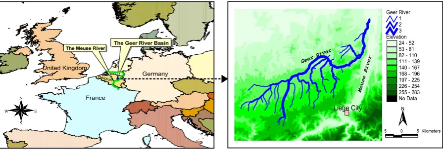
Fig. 3. Location of the Geer river basin and the Geer river network.
properties. In the real world, the variability of soil proper-ties is one of the factors that induce quick subsurface storm flow. Within a REW, the soil column is divided into two lay-ers. The average porosity and saturated hydraulic conductiv-ity of the upper layer are larger than those of the lower layer. It should be pointed out that this division of the soil pro-file does not necessarily coincide with the boundary between the unsaturated and saturated zones as the consequence of varying water table depth. Therefore, the effective porosity of these two zones should be updated in time. Applying a depth-weighted averaging method, the effective porosity of both subsurface zones are given by:
εu =
ε0udup+ε0s yu−dup
yu(ifyu> dup) εu =εu0 (ifyu≤dup)
(35)
εs =εu0 dup−yu+ε0s zsurf −zr−dup zsurf −zr−dup(ifyu < dup)
εs =ε0s(ifyu ≥dup)
(36)
whereεu0 (–) andεs0(–) are the soil porosity of the upper layer and the lower layer of the soil column, respectively;dup(L) is the depth of the upper soil layer. By this parameterisa-tion, in combination with the field capacity threshold, which controls when percolation takes place, the time scales of the flow processes in the two subsurface domains can be better represented.
3 Model application
3.1 Site description
The Geer river basin has been selected for this study. The Geer river is a tributary of the Meuse River, located in Bel-gium (Fig. 3). The drainage area covers about 490 km2. The basin is characterised by a deep groundwater system, which is delimited at the southern end by a ridge separating it from
the Meuse River. The substrata are made up by several lay-ers of chalk stone with low permeability. The groundwa-ter aquifer of the basin consists of Cretaceous chalks with a thickness ranging from a few meters in the south to about 100 m in the north. The aquifer is underlain by a layer of Smectite, which can be regarded as an impervious bot-tom boundary. The unsaturated zone above the aquifer can be up to 40 m. The groundwater catchment does not cor-respond to the surface hydrological divide and extends be-yond the catchment boundaries, thus water most likely flows across the northern topographical divide. Moreover, there is groundwater abstraction from wells and there are drainage galleries in the basin. Spatial data, a DEM with 30 m×30 m resolution, as well as four years (1 January 1993–31 De-cember 1996) of daily rainfall, potential evaporation and dis-charges at the outlet are available.
3.2 Model calibration and sensitivity analysis
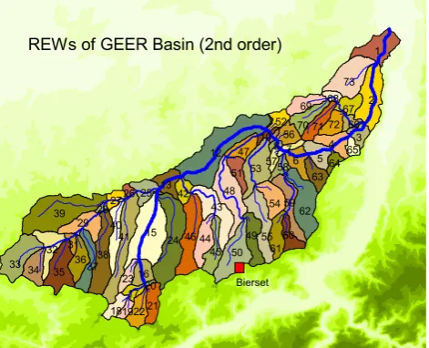
3.2.1 Parameter assignment and manual calibration The river basin has been discretised into a finite number of sub-watersheds, i.e. REWs, and the river network linking each REW has been generated using the modified version of TARDEM (Tarboton, 1997). A second order threshold on the Strahler river order system (Strahler, 1957) resulted in 73 REWs (see Fig. 4). The parameters of the model consist of the interception threshold, surface roughness and channel friction factor, soil properties and hydraulic characteristics. All these parameters are effective values at REW-scale. Ow-ing to the lack of spatially distributed information of these parameters as well as some of the geometric properties, such as the average total soil depth, the depth of the upper soil layer, and the river bed transition layer depth, we assume that they are uniformly distributed over the entire river basin. The initial state of the river basin is also assumed spatially uni-form. As a result, the model functions as a lumped model. On the other hand, it decreases the model parameters to a more manageable number and reduces drastically the cali-bration task, making a quick evaluation of the model at the early development stage possible. For the derivation of initial estimates of soil parameters, we made a realistic guess based on published values (e.g. Troch et al., 1993). Rainfall and potential evaporation (based on Penman-Monteith equation) data, measured at Bierset gauging station (Fig. 4) from 1 Jan-uary 1993 to 31 December 1994 were used in simulation runs for calibration. Discharge data, measured at the outlet of the catchment in the same period were used for calibration. The remaining two years of data were used for verification run. No data measured at interior flow gauges was available. It has been observed that the 4-year of data available for this study cover both wet and dry periods, high and low flows. Further, no drastic changes in climate and land use, which could lead to changes of catchment rainfall runoff relations, have been documented. Therefore, the quantity and quality of the data applied in this case is justified.
Knowing that water flows across the northern divide of the river basin, we imposed a flux boundary condition for those REWs bordering the northern divide (REW12, REW13, REW25, REW26, REW27, REW52, REW69 and REW73). With respect to groundwater abstractions, sink terms have been synthesised as monthly time series on the basis of avail-able data and introduced to the saturated zone mass balance equation for each REW. In addition, groundwater flow inter-actions between neighbouring REWs are considered explic-itly computed with Eq. (18).
It has appeared that the model needs around half a year of run time for model initialisation (warming-up). We there-fore run the model using the time series for one year to reach a quasi dynamic equilibrium state. Subsequently we used this state as the initial state for model calibration so that the warming-up effect can be reduced to a negligible level. By applying a trial-and-error method, expert knowledge has been used to identify parameter values. During manual
cali-12
2
39
15 24
1
41
48
62 46
73
38 50
33
43
4
53 5
55 6
35
59 29
44 49
3
54
32 37
40
45
34 36
70
61
22
71
21
69
13
47
25
63
16
72
60 51
56 67
7
18
42
23
52
27
58
17
66
64 65 8
19
68
57
31
10
26 28
20
REWs of GEER Basin (2nd order)
Bierset
Fig. 4. Discretisation of the Geer river basin and the resultant
REWs.
bration, the most sensitive parameters have been recognised and physically meaningful ranges for those parameters deter-mined. In calibration, two constants, namely the scaling fac-tors,αusandαsf in Eq. (13) and Eq. (23), respectively, were not subject to adjustment. In Eq. (13),αusis the scaling fac-tor resulted from linearisation of the dependent function of the mass exchange between the unsaturated domain and the saturated domain (Reggiani et al., 2000). In this study, sim-ilar to Reggiani et al. (2000), we used the unsaturated soil porosity forαus, implying that the flow (recharge/capillary rise flux) is conducting only through soil pores. As described in Zhang et al. (2005a),ωobeing a function of groundwater level and surface slope, acts, in fact, as a surface runoff coef-ficient. With regard toαsf, we observe that in the right hand side of from Eq. (23), the entire term within the brackets and its exponent vary between 0 and 1. Therefore, αsf should not be larger than the catchment runoff coefficient. For a first estimation ofαsf, the runoff coefficient, and preferably, the surface runoff coefficient can be assigned.
During calibration, priority was given to fitting low flows. While visually inspecting the goodness of fit (comparison of the simulated hydrograph against the observed), objective measures such as the Nash-Sutcliffe efficiency (RNS2 , Nash and Sutcliffe, 1970), the percentage bias (δB)have been used to evaluate the fit. The definition ofRN S2 andδBare given as follows:
RNS2 =1.0−
n
P
i=1
(Qsi−Qoi)2
n
P
i=1
Qoi− ¯Qo2
[image:9.595.311.547.64.255.2]δB =
n
P
i=1
(Qsi−Qoi)
n
P
i=1
Qoi
×100% (38)
whereQsi,QoiandQo¯ are the simulated discharge, the ob-served discharge at the time stepiand the mean of the ob-served discharge, respectively. δB represents the difference of the total volume between the simulated and observed time series. The bias is an important measure to evaluate simula-tion of continuous models.
To give more information on how the model simulates the stream flow in different flow ranges, average relative errors (δp)were calculated.δpis expressed as
δp= 1 n
n
X
i=1
|Qsi−Qoi|
Qoi ×100%
(39)
whereQsiandQoi are the same as in previous equations. 3.2.2 Sensitivity analysis
Sensitivity analysis (SA) is a useful tool to assess the effect of parameter perturbations on model output. Many techniques for SA are available and they can be categorised into three groups (see e.g. Saltelli, 2000): 1) factor screening, 2) local SA, and 3) global SA (often applied as regional sensitivity analysis, RSA, in rainfall-runoff applications). The Fourier amplitude sensitivity test (FAST) and Monte Carlo simula-tion based methods (e.g. Hornberger and Spear, 1981; Beven and Binly, 1992; Freer et al., 1996) are among the popular RSA approaches, which found their applications mostly for conceptual rainfall-runoff models. Apparently, local SA ap-proaches don’t take into account the effect of parameter in-teractions. RSA approaches implicitly account for the pa-rameter interaction effect and can explore a higher dimen-sional parameter space. However, few reports in rainfall-runoff modelling have explicitly discussed the effect of pa-rameter interactions on the papa-rameter indentifiability. In fact, as Bastidas et al. (1999) and Wagener et al. (2004) pointed out, most SA approaches are weak in dealing with the is-sue of parameter interdependency. On the other hand, due to the “curse of dimensionality” (Brun et al., 2001) and pro-hibitively high computational demand, RSA approaches are not widely applied yet to large complex models. Instead, local approaches are often used (e.g. Senarath et al., 2000; Newham et al., 2003).
We used the one-at-a-time perturbation approach to pre-liminarily investigate the effect of parameter variation on the model output that assists in gaining insight into model be-haviour, although sensitivity analysis is not the main goal of this work. This approach can be regarded as an expansion of factor screening that is helpful to filter out most impor-tant factors affecting model response. In this study, starting with the manual calibration, each parameter has been varied
by +50% and−50% while the other parameters were main-tained unchanged. Having gained a knowledge of which pa-rameters are most sensitive in manual calibration, we chose six parameters (idc, Ksu, Kss, εs0, ε
0
u, λ) to further evalu-ate model sensitivity. Using the relative change in runoff volume (δV)and the relative change in Nash-Sutcliffe effi-ciency (δN S)as indices, the effect of each parameter change on the runoff-producing events during the period from 1 Jan-uary 1993 to 31 December 1993 has been analysed. δV and δN Sare defined as follows:
δV =
n
P
i=1
(Qi+−Qi−)
n
P
i=1
Qim
×100% (40)
whereQi+,Qi−andQimrefer to the discharges at the time stepiwith the parameter value varied by +50%,−50% and the manually calibrated parameter value, respectively. The larger theδV, the more sensitive the model is to the parameter under study.
δNS =
R2NS+−R2NS− RNSm2
×100% (41)
whereRNS2 +, R2NS− and RNSm2 are the Nash-Sutcliffe effi-ciency values with the parameter value varied by +50%,
−50% and the manually calibrated parameter value, respec-tively. Same asδV, the larger theδNS, the more sensitive the model to the parameter under study.
3.2.3 Automated parameter optimisation
A hybrid approach combining manual and automated cal-ibration methods is increasingly recognised as a more ef-fective way of parameter optimisation (Boyle et al., 2000). Boyle et al. (2000) first carried out automatic calibration us-ing the MOCOM-UA algorithm to obtain the Pareto solu-tion space and then selected one or more acceptable param-eter sets within the Pareto space through manual calibration. Obviously this calibration strategy has the advantage that a group of good parameter sets can be efficiently filtered out by the automatic step. In our case, however, the model is newly built and further development is still underway. Thus, an open-eyes manual calibration is a desirable way of gain-ing knowledge of model behaviour. Moreover, the model is physically based so that parameters should be calibrated within physically reasonable ranges, which have to be de-fined before an automatic calibration step. Therefore, we carried out manual calibration in the first step followed by automatic calibration.
Table 2. The accepted best parameter values for the calibration period and the model performance.
Parameters idc
(mm/d)
n
(s/m1/3)
Kss
(m/d)
Ksu
(m/d)
Ksr
(m/d)
ε0s
(–)
ε0u
(–)
λ
(–)
θf
(–) Value 1.36 0.020 0.0097 0.0213 2.64 0.148 0.43 4.43 0.08
RNS2 0.71
δB 0.76%
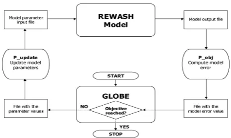
calibration procedure for the fine adjustment of parameter values. In this work, the optimisation tool GLOBE (Solo-matine, 1995, 1998) has been coupled to REWASH. GLOBE is a global optimisation tool consisting of a number of search algorithms: controlled random search (CRS2, CRS4); ge-netic algorithm (GA); adaptive cluster covering (ACCO), and with local search (ACCOL); multistart methods (e.g. M-simplex) etc. We choose the M-simplex algorithm for our study, though Sorooshian et al. (1993) discussed that the M-simplex algorithm is not as efficient and effective as the shuf-fled complex evolution algorithm. In our modelling exer-cises, we also have tried different algorithms (GA, ACCOL). However, the accuracy gained was marginal and the com-putational efficiency was found lower than that with the M-simplex. Figure 5 shows the loop of the automated calibra-tion procedure. P obj and P update are the two programmes linking REWASH to GLOBE. These programmes are driven by GLOBE in each evaluation loop, in which P update takes the values of the parameter set generated from GLOBE and updates the input files for the REWASH, and P obj provides the error value calculated with a specified objective function (i.e.RNS2 for this work) to GLOBE.
3.3 Model verification
Model verification has been performed to test whether the model, using the same parameter set obtained by optimi-sation, but with independent data sets, can produce outputs with reasonable accuracy. A classical method for model ver-ification, the split-sample test (Klemes, 1986) has been ap-plied since there is no indication that there has been an abrupt change of the basin characteristics and conditions over the time domain of the investigation. The data set from 1 Jan-uary 1995 to 31 December 1996 has been used for the veri-fication test. To examine whether the model can perform in a consistent manner in terms of simulating the real system within the range of accuracy, a model validity test has been conducted by reversing calibration and verification periods. In this analysis, the data set of the period from 1 January 1995 to 31 December 1996 is used for calibration while the other part of the data set is used for verification.
Fig. 5. Flow chart of the automatic calibration procedure (after
Solomatine, 1998).
4 Results and discussion
4.1 Model calibration
After manual and automatic calibration with a limited num-ber of parameters (idc, Ksu, Kss, ε0s, ε
0
u, λ), the Nash-Sutcliffe efficiency of the model reached 0.71, while the vol-ume error represented byδB was only 0.76%. Table 2 lists the accepted best parameter values and the model perfor-mance. The values of the saturated hydraulic conductivity of the unsaturated zone and the soil porosity of the upper soil layer are more than twice as high as those of the saturated zone and of the lower soil layer, respectively. Theλvalue indicates that the soil type is silty loam, which agrees with other soil property indicators, such asKsuandεu0.
[image:11.595.311.544.191.330.2]Table 3. Average relative simulation errors in different flow ranges.
Averaged relative errorsδp(%)
Flow (Q) ranges Calibration results Calibration results Verification results (m3/s) (1993–1994) without interception (1995–1996)
(1993–1994)
Q≤1.0 9.7 6.5 –
1.0<Q≤2.0 15.0 17.7 19.8
2.0<Q≤6.0 19.5 24.9 25.4
6.0<Q≤8.0 38.6 41.9 15.9
>8.0 22.2 27.0 36.9
data. However, we argue that these under- and overestima-tion for the peaks are not entirely due to the modelling er-rors but also as result of data erer-rors and the neglecting spa-tial distribution of rainfall. If we examine the rainfall data (Fig. 6a) in the period between day 560 and day 580, there are three rainfall events with relatively high rainfall inten-sity ranging from 11.8 to 24.4 mm/d. These events should have produced higher stream flows than observed. The in-consistency between the rainfall observations and the dis-charge measurements is most likely due to the fact that only one rainfall station was used for the simulation. The flow duration curves (Fig. 7) for the simulated and observed dis-charges show that low flows are better simulated than middle-ranged flows when comparing to the measured data. This is confirmed by Table 3. For low flows (Q≤1.0 m3/s, and 1.0 m3/s<Q≤2.0 m3/s), the averaged relative errors (δp)are 9.7% and 15.0%, respectively. They are significantly smaller than those for flows in the ranges of 2.0–6.0 m3/s and 6.0– 8.0 m3/s, which are 19.5% and 38.6%, respectively. Yet we realise that the model involves parameter uncertainties since there are no catchment-scale parameters ever measured or detailed data on state variables other than discharge to con-firm the calibrated model parameters. This remains a chal-lenge for ongoing and future research.
4.2 Model sensitivity to parameters
A set of computer runs has been implemented to test model sensitivity to parameters listed in Table 4. The analysis pri-marily focused on subsurface parameters. Table 4 shows that runoff simulations are most sensitive to the soil pore-disconnectednessλ and the soil porosity of the lower soil layerεs0.λmostly affects the runoff volume whileεs0 has the strongest effect on the Nash-Sutcliffe efficiency. This can be explained if we recall the equations described in Sect. 2. From Eqs. (10), (14), (15) and (32), we see thatλis the one that determines the unsaturated hydraulic conductivity and the unsaturated zone hydraulic potential, and hence the infil-tration capacity and the percolation flux. From Eq. (33), one can observe thatε0sdictates the subsurface storage and
inter-0 100 200 300 400 500 600 700
0
10
20
30
40
50
a) Observed rainfall at the Bierset gauging station − calibration period
rainfall intensity (mm/d)
daily rainfall intensity
0 100 200 300 400 500 600 700
0 5 10
b) Discharges at the outlet of the Geer river − calibration period
Discharge − (m
3/s)
simulated observed R2NS=0.71
0 100 200 300 400 500 600 700
0 2 4 6 8 10 12x 10
7 c) Cumulative discharges at the outlet of the Geer river − calibration period
time (01/01/1993 −31/12/1994) − (days)
Cumulative discharge − (m
3)
simulated observed δB=0.76%
Fig. 6. Comparison of the simulated and the observed hydrograph
and cumulative discharge volume at the basin outlet for the calibra-tion period (1 January 1993–31 December 1994): (a) the rainfall,
(b) the observed and simulated discharge, (c) the accumulated
ob-served and simulated runoff.
actions between surface and subsurface flows. Meanwhile, these equations also explain the significance ofKss andεu0 in model performance. The test results already suggested a remarkable effect of the interception thresholdidcon runoff generation although it’s sensitivity is smaller than the subsur-face parameters. The effect ofidcis discussed in more details in the following section.
4.3 Effect of interception
[image:12.595.311.545.238.434.2]Stream flow duration curve_calibration
0 2 4 6 8 10
0 20 40 60 80 100
percentage of discharge exceedance
d
is
c
h
a
rg
e
(
m
³/
s
[image:13.595.309.546.63.255.2]) simulated observed
Fig. 7. Flow duration curves for the model calibration results and
[image:13.595.51.283.69.245.2]the observed data.
Table 4. Sensitivity of the model output to parameters.
Parameters δV(%) δNS(%)
λ(–) 190 1177
ε0s(–) 109 1729
Kss(m/d) 81 45
εu0 (–) 77 89
Ksu(m/d) 10 6 idc(mm/d) 10 5
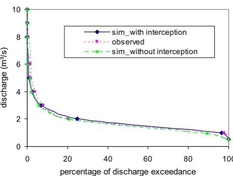
worse than the one with interception:R2N Sis 14% lower, and δB is 187% larger. Figure 9 shows the flow duration curves for the simulation outputs of both the models with and with-out interception, as well as for the observed flow records. To-gether with analysing the averaged relative errorδppresented in Table 3, we can find that the model without interception does not cover the full range of the low flows, suggesting erroneous simulation of the water balance. This is because more water, which would have been intercepted, is adding to the subsurface stores, participating in the surface and subsur-face flux exchanges, and subsequently contributes to stream flow. Especially during the smaller rainfall events, the part of the rainfall flux that would have been intercepted leads to a higher antecedent soil moisture state, which either initiates a quicker surface runoff or gives rise to higher stream flow during the low flow regime. In the simulation without inter-ception, we see that low flows are higher than observed, e.g. in the period of the last 120 days (Fig. 8a). However, as the model tries to maintain overall performance in terms of to-tal volume, the simulated flow mass curve enters into a more or less constant slope, which does not follow the bending of the observed flow mass curve after 360 days (Fig. 8b). In
0 100 200 300 400 500 600 700
0 2 4 6 8 10
a) Discharges at the outlet of the Geer river
time (01/01/1993 − 31/12/1994) − (days)
Discharge − (m
3/s)
simulated− without interception observed
R2NS=0.61
0 100 200 300 400 500 600 700
0 2 4 6 8 10 12x 10
7 b) Cumulative discharges at the outlet of the Geer river
time (01/01/1993 − 31/12/1994) − (days)
Cumulative discharge − (m
3)
simulated − without interception observed
δB=2.2%
Fig. 8. Simulated discharge using the model without interception
after optimisation (1 January 1993–31 December 1994): (a) ob-served and simulated discharge, (b) accumulated obob-served and sim-ulated runoff.
Stream flow duration curve
0 2 4 6 8 10
0 20 40 60 80 100
percentage of discharge exceedance
d
is
c
h
a
rg
e
(
m
³/
s
)
sim_with interception observed
sim_without interception
Fig. 9. Flow duration curves for the model calibration results (with
[image:13.595.99.233.328.416.2]interception and without interception) and the observed data.
Fig. 10, one can notice that without interception, the soil sat-uration is steadily increasing over time (dotted lines) for each of the REWs presented. However, one would expect that for a multiple-year simulation, the soil moisture state would pre-serve an equilibrium state while varying seasonally.
4.4 Model verification
[image:13.595.311.542.340.514.2]0 0.5 1 1.5 2 0.5
0.6 0.7 0.8 0.9 1
a) REW 1
t − (year)
s (−)
without interception with interception
0 0.5 1 1.5 2
0.5 0.6 0.7 0.8 0.9 1
b) REW 53
t − (year)
s (−)
without interception with interception
0 0.5 1 1.5 2
0.5 0.6 0.7 0.8 0.9 1
c) REW 54
t − (year)
s (−)
without interception with interception
0 0.5 1 1.5 2
0.5 0.6 0.7 0.8 0.9 1
d) REW 61
t − (year)
s (−)
[image:14.595.51.284.62.254.2]without interception with interception
Fig. 10. Comparison of the hill-slope soil moisture dynamics
[image:14.595.311.544.64.256.2]simu-lated with and without interception process in the model. REW 53, REW54 and REW 61 compose a hill-slope of the catchment in the southern side of the Geer river.
Table 5. Model performance in the split-sample test runs.
test δB(%) R2NS
calibration (1993–1994) 0.76 0.71 verification (1995–1996) 4.79 0.61 reversed calibration (1995–1996) 4.14 0.65 reversed verification (1993–1994) 3.82 0.68
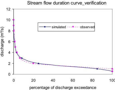
The observed discharge on this day is 9 m3/s and the rainfall causing this peak is 28 mm/d. Scanning all rainfall events and peak responses in the catchment in the period of 1993– 1996, this data point is an exception lying outside the gen-eral rainfall runoff relation of the catchment. It is likely due to either a measurement error or the inadequate density of the rainfall observation network. As a result, it is not used for model performance analysis. In this verification run, low flows in most of the time are underestimated, which can be confirmed from the flow duration curve (Fig. 12). Actually, from Fig. 11b, we can find that the observed flow data exhibit more or less constant base flows and show no remarkable de-pleting trend in the dry period over the time from 1995 to 1996. This appearance is also shown in Fig. 12 in which there is an abrupt change of the probability distribution for the observed discharges from 2.0 m3/s to 1.0 m3/s.
Table 5 reports the summary of the model performance in each of the calibration/verification runs. Figures 13 and 14 present the reversed calibration/verification tests. All these results demonstrate that the model, giving a similar volume error and Nash-Sutcliffe efficiency in each of the simulations, performs in a very consistent manner.
0 100 200 300 400 500 600 700
0
10
20
30
40
50
a) Observed rainfall at the Bierset gauging station − verification period
rainfall intensity (mm/d)
daily rainfall intensity
0 100 200 300 400 500 600 700
0 5 10
b) Discharges at the outlet of the Geer river − verification period
Discharge − (m
3/s) simulated
observed R2NS=0.61
0 100 200 300 400 500 600 700
0 2 4 6 8 10 12x 10
7 c) Cumulative discharges at the outlet of the Geer river − verification period
time (01/01/1995 −31/12/1996) − (days)
Cumulative discharge − (m
3)
[image:14.595.311.543.346.527.2]simulated observed δB=4.8%
Fig. 11. Model verification results: (a) observed daily rainfall
in-tensity at the Bierset station; (b) comparison of the simulated and observed daily discharge at the outlet of the Geer river basin; (c) comparison of the simulated and observed runoff volume (1 Jan-uary 1995–31 December 1996).
Stream flow duration curve_verification
0 2 4 6 8 10 12
0 20 40 60 80 100
percentage of discharge exceedance
d
is
c
h
a
rg
e
(
m
³/
s
) simulated observed
Fig. 12. Flow duration curves for the model verification results and
the observed data.
5 Summary and conclusions
[image:14.595.66.266.353.420.2]0 100 200 300 400 500 600 700 0
2 4 6 8
10 a) Discharges at the outlet of the Geer river − reverse calibration period
time (01/01/1995 − 31/12/1996) − (days)
Discharge − (m
3/s)
simulated observed R2NS=0.65
0 100 200 300 400 500 600 700
0 2 4 6 8 10 12x 10
7 b) Cumulative discharges at the outlet of the Geer river − reverse calibration period
time (01/01/1995 − 31/12/1996) − (days)
Cumulative discharge − (m
3)
[image:15.595.311.545.63.257.2]simulated observed δB=4.1%
Fig. 13. Calibration results by reversing the calibration/verification
periods (1 January 1995–31 December 1996): (a) observed and simulated discharge, (b) accumulated observed and simulated runoff.
principles. To enhance the model’s numerical efficiency and stability, the momentum balance equations have been simpli-fied by ignoring inertia terms, leading to algebraic forms of exchange fluxes. The mass balance equations have been con-verted into univariate derivative form so that a single variable is computed to represent the state of each flow domain at each time step. An adaptive-step-size controlled Runge-Kutta in-tegration algorithm has been applied to solve the coupled sys-tem of equations, ensuring model stability while maintaining accuracy. The model has been coupled to the GLOBE opti-mization tool for automatic calibration.
The model has been applied to the Geer river basin, which lies in a temperate humid climate region. This basin has a complex subsurface where cross-boundary interactions and groundwater flows are essential features. It is further com-plicated by human interference through pumping and artifi-cial underground drainage, giving rise to a great deal of diffi-culty in modelling its hydrological response. Model calibra-tion was carried out using a combined manual and automatic method. The sample-split test resulted in a similar accuracy, suggesting that the model performs in a consistent manner in the study area. Judging by the Nash-Sutcliffe efficiency and volume percentage bias, it can be concluded that the simu-lated stream flows are reasonably accurate.
The introduction of interception in the model, in spite of the simplicity of the approach, showed that it improved the soil moisture accounting, resulting in a better stream flow simulation. Subject to the research objective, a more sophis-ticated module for interception, taking into account the effect of temporal and spatial variation due to vegetation type and their seasonal changes can be further investigated in the fu-ture.
0 100 200 300 400 500 600 700
0 2 4 6 8 10
a) Discharges at the outlet of the Geer river − reverse verification period
time (01/01/1993 − 31/12/1994) − (days)
Discharge − (m
3/s)
simulated observed R2NS=0.68
0 100 200 300 400 500 600 700
0 2 4 6 8 10 12x 10
7 b) Cumulative discharges at the outlet of the Geer river − reverse verification period
time (01/01/1993 − 31/12/1994) − (days)
Cumulative discharge − (m
3)
simulated observed δB=3.8%
Fig. 14. Verification results by reversing the calibration/verification
periods (1 January 1994–31 December 1995): (a) observed and simulated discharge, (b) accumulated observed and simulated runoff.
It is observed that deriving closure relations for mass ex-change terms in the balance equations is the key to a suc-cessful application of the REW approach. In general, clo-sure relations can be deducted from theoretical analysis, nu-merical experiments, field experiments, physical reasoning on intuitive grounds, and a combination of any of the above-mentioned methods (e.g. Lee et al., 2005; Zehe et al., 2005). Taking the advantage of the REW approach for its flexibility, one can opt for an appropriate approach for the derivation of closure relations on a case-by-case basis, putting empha-sis on those closure relations that are most relevant for the dominant processes in the catchment under study.
This paper demonstrates that the model, REWASH, pre-sented here is capable of capturing watershed responses and simulating rainfall-runoff behaviour. Although there is still substantial work to be done before the model can be routinely applied in catchments with different physio-geographic and climatic settings, REWASH provides a general framework as an alternative for physically based distributed modelling ap-proaches. One can tune this model or modify any functional relation to suite the characteristics of a specific study site.
Appendix: Nomenclature
Dimensions:L=length;T=time;M=mass.
A horizontally projected surface area of a REW (L2).
dup depth of the upper soil layer (L). ep potential evaporation (LT−1). ect op,eot op,
ert op
[image:15.595.51.284.64.256.2]eca,ecu,eco interception flux from Czone, infiltration flux to Uzone, flux between Czone and Ozone (L3T−1).
eoa, eos, eor, eoc
evaporation flux from Ozone, flux be-tween Ozone and Szone, flux bebe-tween Ozone and River, flux between Ozone and Czone (L3T−1).
eua,euc,eus transpiration fux in Uzone, infiltration flux from Czone, percolation flux to Szone (L3T−1).
esu,eso the counterpart ofeusandeso.
esr,esi,esa flux between Szone and River, flux ex-change between the neighbouring REWs, groundwater abstraction (L3T−1). era,erin,erout evaporation from River, flux from
up-stream River, flux to the downup-stream River (L3T−1).
ers,ero the counterpart ofesrandeor. f infiltration capacity (L3T−1).
g gravitational acceleration (LT−2). G groundwater abstraction or recharge rate
(L3T−1).
hc capillary pressure head (L).
ho, hr,hs total hydraulic head for Ozone, River and Szone (L).
i precipitation intensity (LT−1).
idc interception threshold for Czone (LT−1). Ksu,Ku saturated and effective hydraulic
conduc-tivity for Uzone (LT−1).
Ksr,Kss saturated hydraulic conductivity for riverbed and Szone (LT−1).
lr length of the river channel (L). m average cross-sectional area (L2). n Manning roughness coefficient (TL1/3). Pr wetted perimeter of the river cross section
(L).
Qsi,Qoi,Q¯o simulated discharge, observed discharge at the time step i,mean of the observed discharge (L3T−1).
Qi+,Qi−,
Qim
discharges after the parameter perturba-tion by ±50% at time step i, discharge after the accepted manual calibration at time stepi(L3T−1).
RNS2 Nash-Sutcliffe efficiency (–). RNS2 +, R2NS−,
RNSm2 ,RNS2
values after parameter perturbation by
±50%, and after the accepted manual cal-ibration (–).
s sink or source term.
Sc,So,Su,Ss, Sr
storage of Czone, Ozone, Uzone, Szone and River (M).
vo,vr velocity of the flow in the River and Ozone (LT−1).
wr width of the river channel (L).
yo depth of flow sheet over the overland flow zone surface (L).
yr water depth of the river channel (L). ys,yu average depth of Szone and Uzone (L). zr,zs,zsurf average elevation for river bed, ground
surface and soil bottom (L). Z average soil depth (L).
αsf scaling factor for Ozone area computa-tion (–).
αsi lumped scaling factor for regional groundwater flow (L2T−1).
αus scaling factor for flux exchange between Uzone and Szone (–).
δB discharge volume percentage bias (–). δNS relative change in Nash-Sutcliffe
effi-ciency (–).
δV relative change in percentage bias (–). δp average relative error (–).
ε0u,ε0s porosity of the upper and lower soil layer (–).
εu,εs effective soil porosity of Uzone and Szone (–).
φ generic thermodynamic property. γo average surface slope angle of Ozone in
radian.
γr average slope angle of the channel bed in radian.
λ soil pore-disconnectedness index (–). 3r depth of the transition zone of the river
bed for the base flow (L).
3s typical length scale for the exfiltration flux (seepage) (L).
3u length scale of the wetting front for infil-tration (L).
µ soil pore size distribution index (–). θf field capacity of Uzone (–). ρ water density (ML−3).
ωo,ωc,ωo area fraction of the saturation-excess overland flow domain, infiltration-excess flow domain and the unsaturated flow do-main (–).
ξ Darcy-Weisbach friction factor for the channel routing (–).
ψb air entry pressure head at Uzone (L).
Acknowledgements. This research has been funded by the Delft
by E. Zehe, an anonymous referee and the editor, M. Sivapalan have considerably improved the manuscript. It is highly ap-preciated that P. Reggiani provided the original computer code, based on which the numerical model REWASH has been developed. Edited by: M. Sivapalan
References
Abbott, M. B., Bathurst, J. C., Cunge, J. A., O’Connell, P. E., and Rasmussen, J.: An introduction to the European Hydrologic Sys-tem SysSys-teme Hydrologique Europeen, SHE, 1: History and phi-losophy of a physically based, distributed modelling system, J. Hydrol., 87, 45–59, 1986a.
Abbott, M. B., Bathurst, J. C., Cunge, J. A., O’Connell, P. E., and Rasmussen, J.: An introduction to the European Hydrologic Sys-tem SysSys-teme Hydrologique Europeen, SHE, 2: Structure of a physically based, distributed modelling system, J. Hydrol., 87, 61–77, 1986b.
Bastidas, L.A., Gupta, H. V., Sorooshian, S., Shuttleworth, W. J., and Yang, Z. L.: Sensitivity analysis of land surface scheme us-ing multicriteria methods, J. Geophys. Res., 104, 19 481–19 490, 1999.
Bergstr¨om, S. and Forsman, A.: Development of a conceptual de-terministic rainfall-runoff model, Nordic Hydrol., 4, 147–170, 1973.
Bergstr¨om, S.: The HBV model, in: Computer models of watershed hydrology, edited by: Singh, V. P., Water Resources Publications, USA, 443–520, 1995.
Beven, K. J.: Infiltration into a class of vertically non-uniform soils, Hydrol. Sci. J., 29, 425–434, 1984.
Beven, K. J.: Changing ideas in hydrology: the case of physically based models, J. Hydrol., 105, 157–172, 1989.
Beven, K. J.: Prophesy, reality and uncertainty in distributed hydro-logical modelling, Adv. Water Res., 16, 41–51, 1993.
Beven, K. J.: A discussion of distributed hydrological modelling, in: Distributed hydrological modelling, edited by: Abbott, M. B. and Refsgaard, J. C., Kluwer Academic Publishers, Dordrecht, The Netherlands, 255–278, 1996a.
Beven, K. J.: Response to comments on “A discussion of distributed hydrological modelling” by Refsgaard, J. C. et al., in: Distributed hydrological modelling, edited by: Abbott, M. B. and Refsgaard, J. C., Kluwer Academic Publishers, Dordrecht, The Netherlands, 289–295, 1996b.
Beven, K. J.: Equifinality and uncertainty in geomorphological modelling, in: The scientific nature of geomorphology, edited by: Rhoads, B. L. and Thorn, C. E., John Wily & Sons, Chich-ester, UK, 289–313, 1996c.
Beven, K. J.: Towards an alternative blueprint for a physically based digitally simulated hydrologic response modelling system, Hy-drol. Process., 16, 189–206, 2002.
Beven, K. and Binly, A.: The future of distributed models: model calibration and uncertainty predication, Hydrol. Process., 6, 279– 298, 1992.
Beven, K. J., Calver, A., and Morris, E.: The Institute of Hydrology distributed model, Institute of Hydrology Report No. 98, UK, 1987.
Beven, K. J., Lamb, R., Quinn, P., Romanowicz, R., and Freer, J.: TOPMODEL, in: Computer models of watershed
hydrol-ogy, edited by: Singh, V. P., Water Resources Publications, USA, 627–668, 1995.
Bl¨oschl, G. and Sivapalan, M.: Scale issues in hydrological mod-elling – a review, Hydrol. Process., 9, 251–290, 1995.
Boyle, D. P., Gupta, H. V., and Sorooshian, S.: Toward improved calibration of hydrologic models: Combining the strengths of manual and automatic methods, Water Resour. Res., 36, 3663– 3674, 2000.
Brooks, R. H. and Corey, A. T.: Hydraulic properties of porous media, Hydrol. Pap. No. 3, Colorado State Univ., Fort Collins, 1964.
Brun, R., Reichert, P., and K¨unsch H. R.: Practical identifiability analysis of large environmental simulation models, Water Re-sour. Res., 37, 1015–1030, 2001.
Burnash, R. J. C., Ferral, R. L., and McGuire, R. A.: A Generalized streamflow simulation system – Conceptual modeling for digi-tal computers, US Department of Commerce, National Weather Service and State of Califonia, Department of Water Resources, 1973.
Burnash, R. J. C.: The NWS river forecast system – Catchment modelling, in: Computer models of watershed hydrology, edited by: Singh, V. P., Water Resources Publications, USA, 311–366, 1995.
Calver, A and Wood, W. L.: The Institute of Hydrology distributed model, in: Computer models of watershed hydrology, edited by: Singh, V. P., Water Resources Publications, USA, 595–626, 1995.
Cash, J. R. and Karp, A. H.: ACM Transactions on Mathematical Software, 16, 201–222, 1990.
Doorenbos, J. and Kassam A. H.: Yield response to water, FAO irrigation and drainage paper 33, Food and Agriculture Organi-sation, Rome, 1979.
Dunne, T. and Black, R. D.: Partial area contributions to storm runoff in a small New England watershed, Water Resour. Res., 6, 1296–1311, 1970.
Dunne, T.: Field studies of hillslope flow processes, in: Hillslope Hydrology, edited by: Kirkby, M. J., John Wily & Sons, Chich-ester, UK, 227–293, 1978.
Freer, J., Beven, K., and Ambroise, B.: Bayesian estimation of un-certainty in runoff prediction and the value of data: An applica-tion of the GLUE approach, Water Resour. Res., 32, 2161–2173, 1996.
Freeze, R. A. and Harlan, R. L.: Blueprint for a physically-based, digitally-simulated hydrologic response model, J. Hydrol., 9, 237–258, 1969.
Grayson, R. B., Moore, I. D., and McMahon, T. A.: Physically based hydrologic modeling, 1, A terrain-based model for inves-tigative purposes, Water Resour. Res., 28, 2639–2658, 1992a. Grayson, R. B., Moore, I. D., and McMahon, T. A.: Physically
based hydrologic modeling, 2, Is the concept realistic?, Water Resour. Res., 28, 2659–2666, 1992b.
Hewlett, J. D. and Hibbert, A. R.: Factors affecting the response of small watersheds to precipitation in humid areas, in: Proceedings of 1st International Symposium on Forest Hydrology, edited by: Sopper, W. E. and Lull, H. W., Pergamon, 275–290, 1967. Hornberger, G. M. and Spear, R. C.: An approach to the preliminary