1b . Note the initial estimated position does not appear to be

ECE-520: Linear Control Systems Homework 8

Due: Thursday February 2 at 5 PM

In this homework we will simulate and study the current full order observer coupled with state variable feedback, and then we will add on integral control.

The current observer tries to utilize the most recent data possible. How this type of observer actually works in a given system depends on when the sampling in the system takes place.

Our systems (with the delay) will not work with the current observer, so we will have to simulate systems without delays.

For the first four problems, utilize the torsional system models available from the class website.

1a) Copy your program DT_sv1_observer_driver.m to DT_sv1_current_obs_driver.m You will need to modify the part of the code that determines the observer gains, and you will have to have the program call the simulation DT_sv1_current_observer.mdl. Copy the Simulink file DT_sv1_observer.mdl to DT_sv1_current_observer.mdl . Modify this new file to implement state variable feedback using a full order current observer to estimate the states for a one degree of freedom system. Since the current observer does not work for our systems with delays, you will need to modify to model to have only two state variables. Note that if our system has no integrator in it, there should be a prefilter. Be sure is taken to be the signal just before the limiter. Be sure you use the estimated states (the states feeding into the G in the current observer.)

( ) u k

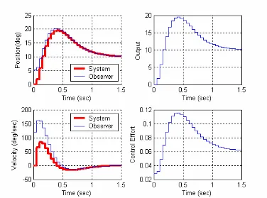
b) Place both the state feedback and observer poles all at 0.7. The output of the system is the position of the first disk and this is also the output available to the observer ( in this case). The disk is initially estimated to be at 10 degrees (be careful of units here! The model works in radians.). The initial estimates of the velocity and delayed control signal are zero. The real system starts at rest (all initial conditions are zero.) For a 10 degree step input you should get the graph shown in Figure 1. Turn in your plot.

y C=C

Figure 1. Results for problem 1b. Note the initial estimated position does not appear to be 10 degrees, and the initial estimated velocity is not zero.

2a) Copy your program DT_sv2_observer_driver.m to DT_sv2_current_obs_driver.m You will need to modify the part of the code that determines the observer gains, and you will have to have the program call the simulation DT_sv2_current_observer.mdl. Copy the Simulink file DT_sv2_observer.mdl to DT_sv2_current_observer.mdl . Modify this new file to implement state variable feedback using a full order current observer to estimate the states for a two degree of freedom system. Since the current observer does not work for our systems with delays, you will need to modify to model to have only four state variables. Note that if our system has no integrator in it, there should be a prefilter. Be sure is taken to be the signal just before the limiter. Be sure you use the estimated states (the states feeding into the G in the current observer.)

( ) u k

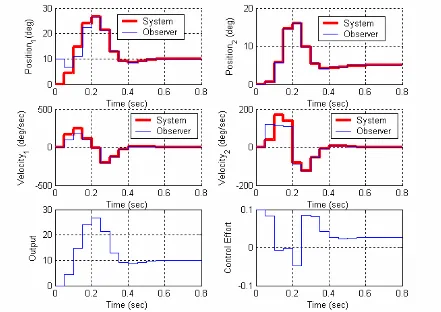
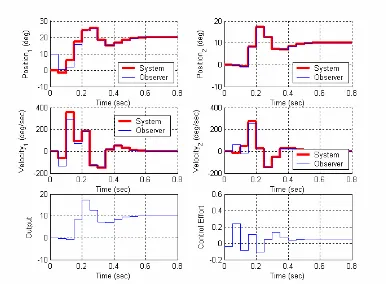
b) Place all the state feedback poles at 0.2, and the observer poles at 0.1. Assume the position of the second disk is available to the observer and the system output is the position of the first disk. The velocities of the disks are initially estimated to be zero. The estimated position of the first disk is assumed to be 10 degrees and the estimated position of the second disk is assumed to be 0 degrees. The real system starts at rest. For a 10 degree step input you should get the graph shown in Figure 2. Turn in your plot.

0.08, 0.1, and 0.12 (you’ll need to use the place command.) You should get the results shown in Figure 3. Turn in your plot.

Figure 3: Results for problem 2c.

3) Now we want to combine the current observer and state feedback with integral control for the one degree of freedom system. We will continue to utilize the torisional model we have been using.

a) Copy your program DT_sv1_obs_servo_driver.m to

DT_sv1_current_obs_servo_driver.m You will need to modify the part of the code that determines the observer gains, and you will have to have the program call the simulation DT_sv1_current_obs_servo.mdl. Copy the Simulink file DT_sv1_obs_servo.mdl to

DT_sv1_current_obs_servo.mdl . Modify this new file to implement state variable feedback using a full order current observer to estimate the states for a one degree of freedom system. Since the current observer does not work for our systems with delays, you will need to modify to model to have only two state variables. Note that our system has an integrator in it, so there should be no prefilter. Be sure is taken to be the signal just before the limiter. Be sure you use the estimated states (the states feeding into the G in the current observer.)

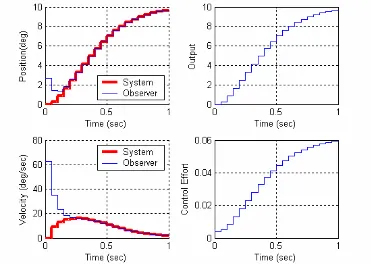
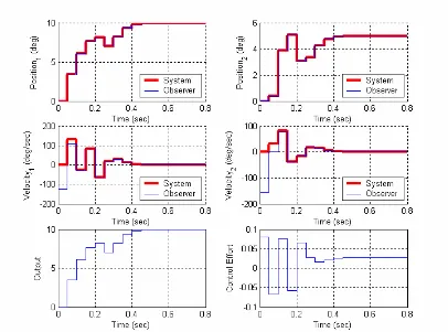
b) Place all the state feedback poles at 0.7 and all of the observer poles at 0.5. The output of the system is the position of the first disk and this is also the output available to the observer ( in this case). The disk is initially estimated to be at 10 degrees, the velocity is initially estimated to be 0 degrees. The true system is initially at rest (all initial states are zero) For a 10 degree step input you should get the graph shown in Figure 4. Turn in your plot.

y C=C

4) Finally, we want to combine the observer and state feedback with integral control for the two degree of freedom system. We will continue to utilize the torisional model we have been using.

a) Copy your program DT_sv2_obs_servo_driver.m to

DT_sv2_current_obs_servo_driver.m You will need to modify the part of the code that determines the observer gains, and you will have to have the program call the simulation DT_sv2_current_obs_servo.mdl. Copy the Simulink file DT_sv2_obs_servo.mdl to

DT_sv2_current_obs_servo.mdl . Modify this new file to implement state variable feedback using a full order current observer to estimate the states for a two degree of freedom system. Since the current observer does not work for our systems with delays, you will need to modify to model to have only four state variables. Note that our system has an integrator in it, so there should be no prefilter. Be sure is taken to be the signal just before the limiter. Be sure you use the estimated states (the states feeding into the G in the current observer.)

( ) u k

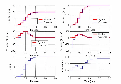
b) Place all the state feedback poles at 0.1, and the observer poles all at 0.06, 0.08, 0.1, and 0.12. Assume the position of the second disk is available to the observer and the system output is the position of the second disk. The estimated position of the first disk is assumed to be 10 degrees all other initial estimates are zero. The real system starts at rest. For a 10 degree step input you should get the graph shown in Figure 5. Turn in your plot.

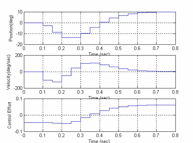
c) For the same conditions as part b, but assume the position of the second disk is available to the observer and the system output is the position of the first disk. The estimated position of the first disk is assumed to be 10 degrees all other initial estimates are zero. The real system starts at rest. Simulate the system for a 10 degree step. You should get a graph like that shown in Figure 6. Turn in your plot.

d) For the same conditions as part c, but assume the position both disks is available to the observer and the system output is the position of the first disk. The estimated position of the first disk is assumed to be 10 degrees all other initial estimates are zero. The real system starts at rest. Simulate the system for a 10 degree step. You should get a graph like that shown in Figure 7. Turn in your plot.

e) For the same conditions as part c, but assume the position of the first disk is available to the observer and the system output is the position of the second disk. The estimated position of the first disk is assumed to be 10 degrees all other initial estimates are zero. The real system starts at rest. Simulate the system for a 10 degree step. How well does the system work? Try

reducing the initial condition until the system seems to work acceptably. Turn in your plot for a case that works well.

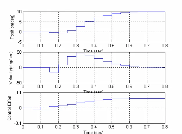
Figure 5: Results for problem 4b.

5) If we want to use the observer/controller in a single input /single output (SISO) control system, we can either put the controller in the feedforward loop or feedback loop, as shown below. Here is the observer controller transfer function, is the transfer function of the plant we are trying to control, and and are prefilter gains (to adjust the step

responses). ( ) oc

G z G z_p( )

A

P P_B

( ) p G z A

P

( )

P

a) Show that if we want these systems to track a step input with zero position error, we should choose the prefilter gains as

1 1 (1) (1) A p oc P G G = + and 1 (1) (1) B oc p P G G = +

Hint: For zero position error the closed loop transfer function should equal 1 when z = 1

b) For the torsional system we have been using, assume the position of the cart is the output and is available to the observer, the feedback poles are all at 0.4, and the observer poles are all at 0.2. We will be looking at a 10 degree step input assuming the system is at rest. Utilizing the Simulink models DT_TF1_A.mdl and DT-TF1_B.mdl show that when you utilize the

observer-controller transfer function (with the prediction full order observer) you get the results displayed in Figures 8 and 9.

The following segments of Matlab will help you construct what you need…. %

% make the transfer function %

GG = G-Ke*C-H*K; HH = Ke;

CC = K; DD = 0;

disp('Poles of the controller are') roots(den_Gc)

%

% set the prefilter gain

determine the plant transfer fucntion

um_Gp,den_Gp] = ss2tf(G,H,C,D);

1 = sum(num_Gc)/sum(den_Gc); %

% % [n % Gc

Gp1 = sum(num_Gp)/sum(den_Gp); Gpf_A = 1 + 1/(Gc1*Gp1);

Gpf_B = Gc1+1/Gp1;.