7.2.1 Digital Carrier Modulation Architecture

7 Digital

Modulation

7.1 Introduction

Once the system designer is faced with the transmission of digital data, the choice of modulation format becomes the primary consideration. This choice is not, however, merely an academic exercise. There are myriad implications for spectrum and spectral efficiency, implementation complexity, power efficiency, and flexibility that the designer must consider. In most cases, the system engineer works within the constraints of the link budgets, cost and complexity, spectrum regulations, and packaging concerns to select the proper modulation format.

This chapter presents the various forms of digital modulation in common use. Special emphasis in placed on visualized the time waveforms and PSDs for each of the formats so that performance can be understood. The chapter ends with a discussion of the various performance measures used to compare and select modulation formats.

7.2 Digital Modulation Principles

Digital modulation schemes differ significantly from analog schemes, primarily in the goal of the communication system. In analog systems, the message waveform is to be preserved through demodulation. In digital systems, only the information is to be preserved; preservation of the message waveform is not a design goal. So choosing a digital modulation format is not about choosing a waveform that will be preserved in transmission and reception, but rather a waveform which will optimally preserve the information in transmission and reception.

At the same time, the choice of a modulation format for digital transmission will be influenced by the ability to maximize data throughput in a limited transmission

bandwidth. This ability is measured by a figure of merit called the spectral efficiency of the modulation format and will be discussed later in the chapter.

Digital modulation formats are classified as binary or multilevel signaling formats. The simplest formats are called binary signaling formats. Binary digital modulations formats not simply subsets of multilevel formats, but are rather formats used exclusively as binary formats. These are analog modulation formats (amplitude, phase, frequency or quadrature modulation) with baseband binary linecode messages having rectangular bit symbol pulses. These modulation formats can possess rather wide transmission bandwidths. One way to reduce the transmission bandwidth is to reduce the message bandwidth. Changing the bit symbol pulse shape can achieve this goal, and this process applied to digital signaling is known as pulse shaping.

modulation stage is the distinguishing feature of this type of signaling. This type of format allows for increased throughput through a bandlimited channel. Pulse shaping is also applied frequently for multilevel digital modulation.

7.2.1 Digital Carrier Modulation Architecture

A typical digital transmitter and receiver design was shown in Chapter 6. In these discussions, we deal with coherent demodulation architectures only, although many of the conversation points apply directly to incoherent receiver structures as well.

The waveform consisting of a line code representation of data bits is the input to the modulator in the transmitter. In fact, this process is an analog modulation process. But since the information transmitted is representative of digital bits, we call it digital modulation. While the operation is identical to what has been discussed before, the formats and results are a bit different.

Whereas analog modulation schemes have been traditionally termed “modulation”, digital modulation schemes, otherwise identical in operation, are term “keying”, denoting the on-off nature of the modulation. (This term traces back to telegraphy.) Thus, DSB-SC with an analog message is called amplitude modulation, while the same DSB-SC

transmission with a digital message is called “on-off keying”.

Frequency upconversion, amplification, and filtering follow the modulation step, and the signal is transmitted. From the signal design perspective, we are concerned mostly with data rate capacity and transmission bandwidth for the transmitted signal. Of course, in transmission, the digitally modulated carrier is just an analog signal, subject to the same constraints and ill effects as any other signal.

In the receiver, the signal is first amplified and downconverted in the RF front end. The received signal is characterized by typical signal parameters such as its SNR and

distortion measures. However, reconstructing either the transmitted waveform or the line code is not the goal of the digital receiver. The carrier modulation format and original line code input to the modulator are typically used and discarded as the signal is processed through the IF stage and demodulator. The final stage of the

receiver/demodulator includes a decision function which must output a line code representation of bits – where each bit estimate is made based upon the waveform received during the corresponding bit interval. Ultimately, a baseband detection problem remains at the end of the signal processing chain.

7.2.2 Binary Digital Modulation

Binary digital modulation schemes arise by applying a binary “digital” waveform as input to an analog modulator. These modulation formats have proven quite effective as a means of transmitting digitized information in noisy environments where analog formats would fail.

configurations, corresponding to a logical “1” or “0”. It will be important to define notation throughout the following discussion. The input bitstream of digital information is clocked at a data rate DR bits per second (bps). The bit interval, or the time duration corresponding to one bit, is denoted Tb seconds. In the transmitted waveform, the

symbols are transmitted at a rate SR symbols per second (sps), and the symbol interval is Ts seconds. For binary modulation, the bit rate and symbol rate are identical. The

transmission bandwidth is BT Hertz.

7.2.2.1 Binary Modulation Waveforms and Spectra

Just as was discussed for amplitude modulation, we can imagine a “digital” message waveform modifying (modulating) a carrier. The same possible carrier modifications are available:

( )

( )

{

( )

( )

}

g t =A t π⎡_⎣f + ∆f t ⎤_⎦t+θ t . (7-1)

The line code waveform could modify the carrier amplitude, frequency deviation, or phase. For binary digital message signals, the message waveforms have the

characteristics of being nearly discreet-valued and discontinuous. This has great impact on the transmitted signal spectrum and receiver performance. Once these characteristics are understood, the system designer can choose the optimum signal waveform for a given application.

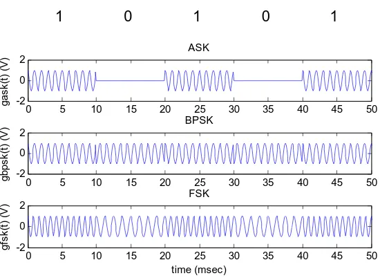
The various modulation formats are displayed as time domain waveforms in Figure 1. In each case, we assume a 100 bps random data input sequence modulating a 1 kHz cosine carrier. The analytic results follow the discussion in Couch [1].

0 5 10 15 20 25 30 35 40 45 50 -2

0 2

ASK

g

a

sk(

t)

(

V

)

0 5 10 15 20 25 30 35 40 45 50 -2

0 2

BPSK

gbps

k

(t

) (

V

)

0 5 10 15 20 25 30 35 40 45 50 -2

0 2

FSK

gf

s

k

(t

) (V

)

time (msec)

Transmitted Digital Modulation Waveforms

1 0 1 0 1

The simplest form of digital carrier modulation is Amplitude-Shift-Keying (ASK), the digital version of DSB-SC. When message is a unipolar line code, the message shifts the carrier amplitude between some positive value and zero (or on and off). In this case the signaling is called On-Off Keying (OOK). This was used first for Morse code

transmission and thus precedes analog message transmission. The OOK waveform is shown as the first waveform in Figure 1. This waveform is particularly easy to detect by first passing the received signal through a bandpass filter centered at the carrier frequency and then passing that output through an envelope detector. The output thus produced is a linecode ready for baseband detection. The chief disadvantage of this format is that amplitude modulation produces a wide transmission bandwidth, as will be demonstrated shortly. The model for an ASK/OOK waveform is

( )

( ) ( )

ASK c

g t =Am t ωt , (7-2)

where m(t) is the unipolar linecode message waveform.

Another binary modulation format is Binary Phase-Shift Keying (BPSK), which can be thought of as phase modulation with the input waveform being a unipolar linecode waveform. The carrier phase is typically shifted from 0° to 180°. This is demonstrated in the second waveform of Figure 1. In this waveform, there is a phase discontinuity at the linecode discontinuities (bit transitions). BPSK can be also be modeled as ASK (DSB-SC) with a polar linecode message. Using this model, both OOK and BPSK may be viewed as holding the frequency and phase of the carrier constant while the amplitude is shifted.

In Frequency Shift Keying (FSK), the carrier amplitude is held constant, and the

frequency is shifted between two frequencies according to the input message. Normally, the input message is a unipolar line code. The amount of frequency shift away from the unmodulated carrier frequency is called the frequency deviation. There are two types of FSK, discontinuous-phase FSK and continuous-phase FSK. In discontinuous-phase FSK, the carrier frequency is directly shifted from one frequency to another according to the binary data (via ∆f). This technique is normally not used, due to the amplitude

fluctuations that accompany the modulation.

The continuous-phase FSK technique is shown in the third waveform of Figure 1. Note that the phase of the waveform is continuous as the name suggests. Also note the constant-envelope nature of the waveform. In this modulation format, the message is set equal to an instantaneous frequency deviation, which is integrated to produce the carrier instantaneous phase. The model for continuous-phase FSK is

( )

( )

CP FSK c f

g ₋ t = A _⎣⎡ωt+ π

∫

The term kf is called the peak frequency deviation and determines the shift in frequency when keying. A term often used to describe the frequency deviation for digital

2 k_f h

DR ⋅

= . (7-4)

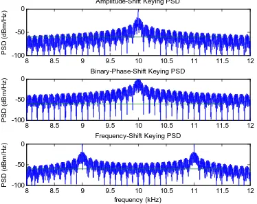
One of our interests in evaluating these modulation formats is to examine their spectra, and to determine the transmission bandwidth required to send data. The transmitted signal power spectral density (PSD) for each of these formats is shown in Figure 2. In each case, narrowband modulation is simulated with a bit/symbol period of 10 msec (DR=100 bps) and a carrier frequency of 10 kHz.

8 8.5 9 9.5 10 10.5 11 11.5 12

-100 -50 0

Amplitude-Shift Keying PSD

PS

D

(

d

Bm

/H

z

)

8 8.5 9 9.5 10 10.5 11 11.5 12

-100 -50 0

Binary-Phase-Shift Keying PSD

PS

D

(

d

B

m

/H

z

)

8 8.5 9 9.5 10 10.5 11 11.5 12

-100 -50 0

Frequency-Shift Keying PSD

frequency (kHz)

PS

D

(

d

Bm

/H

z

)

Figure 2 Power Spectral Density of the three basic binary digital modulation formats: ASK, BPSK, and FSK.

The PSD for OOK is the conventional DSB spectrum for a rectangular pulse-type random message. BPSK however, has much broader sidelobe content due to its nonlinear

modulation mechanism (reminiscent of FM). While its mainlobe (90% power)

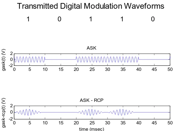
The pulse-shaping technique is often applied to the OOK format to reduce the signal bandwidth, specifically the sidelobe content. An example waveform is illustrated in Figure 3, where a raised-cosine pulse shape is applied to the baseband linecode data prior to modulation. The raised-cosine pulse shape provides advantage in both ISI

management and bandwidth limitation. This produces a shaped-pulse symbol and the shaping is retained in the transmitted modulated carrier.

0 5 10 15 20 25 30 35 40 45 50 -2

0 2

ASK

g

a

sk(

t)

(

V

)

0 5 10 15 20 25 30 35 40 45 50 -2

0 2

ASK - RCP

gas

k

-r

c

p(

t)

(

V

)

time (msec)

Transmitted Digital Modulation Waveforms

1 0 1 1 0

Figure 3 Example of ASK modulation using Raised-Cosine-Pulse-shaped baseband pulses for ISI management and bandwidth reduction.

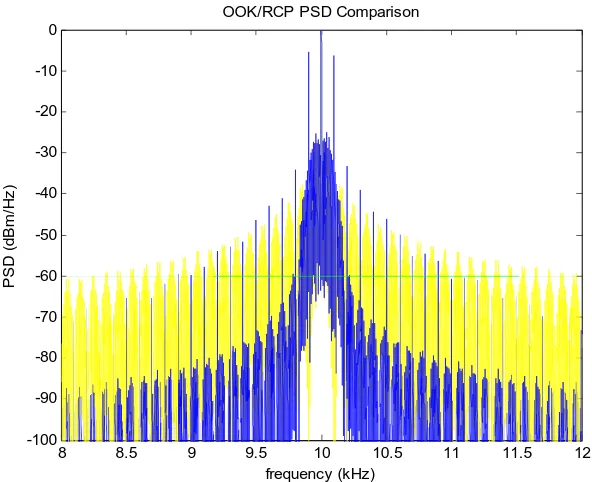
The impact to transmission bandwidth is evident in the power spectral density

8 8.5 9 9.5 10 10.5 11 11.5 12 -100

-90 -80 -70 -60 -50 -40 -30 -20 -10 0

OOK/RCP PSD Comparison

PSD

(

d

Bm

/H

z

)

frequency (kHz)

Figure 4 Transmission spectra for OOK and OOK with raised cosine pulse shaping. Note the dramatic reduction in sideband content resulting from the pulse shaping.

7.2.3 Multilevel Digital Modulation

More advanced digital modulation schemes are available when the designer wishes to greatly increase the data throughput of the system given a fixed bandwidth. This is especially appropriate for wireless systems, where the demand for throughput increases continuously, but the transmission bandwidth allocations increase only sporadically. In the following, a class of multilevel digital signaling is introduced. That is to say that each baseband symbol represents 2m bits of information, where m is an integer greater than 2. Often, these forms of signaling are called m-ary signaling to emphasize this fact. The representation of multiple bits per symbol is performed pre-modulation, and typically quadrature modulation is used to further increase the efficiency of the transmission.

7.2.3.1 QPSK and its Relatives

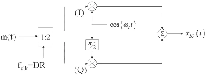
One important multilevel technique involves the use of binary signaling combined with quadrature multiplexing, which results in the class of digital modulation called

Quadrature-Phase-Shift-Keying (QPSK). Each of these important modulation techniques are based on the same modulation architecture, but have important implementation and performance details.

Figure 5 QPSK modulator showing single bitstream feed.

In standard QPSK, a symbol is formed when a symbol derived from the I channel

modulates the amplitude of cosine component of the carrier, and simultaneously a symbol derived from the Q channel modulates the sine component. The baseband symbol

waveform in this case is a standard polar NRZ rectangular pulse waveform. Note that the symbol rate for QPSK is one-half the input serial bitstream bit rate due to the action of the demux.

In Offset QPSK (OQPSK), a delay of ½ of a symbol period (or 1 bit period) is introduced on the Q input to the quadrature modulator. This format is also known as staggered QPSK. This provides an advantage in reducing the residual amplitude modulation on the transmitted signal. [1] (This results because the I and Q data cannot change

simultaneously)

Further reduction of amplitude fluctuations is possible through the use of π/4-shifted QPSK modulation. In this technique, the signaling is performed by alternatively

choosing symbols from the QPSP and OQPSK signal sets. While this seems complicated, it is actually implemented via an algorithm assigning the input bit stream to symbols according to a predefined pattern.

7.2.3.2 Minimum Shift Keying

Another modulation format for improved spectral performance is minimum shift keying (MSK), which modifies the concept of FSK in such a way to improve spectral efficiency and noise performance [2]. MSK can be an m-ary modulation format, but for this

discussion, we will focus on binary MSK.

As indicated above, phase and frequency shift keying can result in rather wide bandwidth transmission signals. MSK offers reduced PSD sidelobe content, and thus reduced

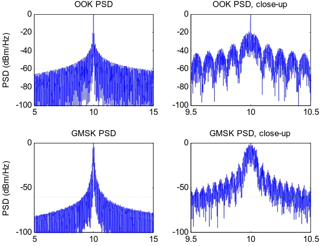
A comparison of the spectral performance of OOK and MSK is given in Figure 6. It is noted that sidelobe content is greatly reduced for the MSK format relative to OOK, which makes MSK so attractive.

5 10 15

-100 -80 -60 -40 -20 0 OOK PSD PSD ( d Bm /H z )

9.5 10 10.5 -100 -80 -60 -40 -20 0

OOK PSD, close-up

5 10 15

-100 -50 0 GMSK PSD PSD ( d Bm /H z )

9.5 10 10.5 -100

-50 0

GMSK PSD, close-up

Figure 6 Comparison of ASK and MSK spectrum for 100 bps bit rate, 10 kHz carrier frequency. A closeup view of the PSDs is shown on the right.

Of course, there is a price to pay, and that is in the receiver. The difficulty in

distinguishing between the small difference in frequency between the two symbols makes the receiver design challenging. However, the engineering has been solved well enough that variations of this modulation method are now extremely popular.

MSK can be modeled as OQPSK where the rectangular symbol pulses have been replaced by half-cycle sinusoidal pulses during the bit interval [1]:

( )

( ) ( ) ( ) ( )

( )

( )

cos sin

cos 1 , sin 1

2 2

msk c c

b b

g t x t t y t t

t

x t A y t A

T T ω ω t π π = − ⎛ ⎞ ⎛ = _⎜± _⎟ = _⎜± _⎟ ⎝ ⎠ ⎝ ⎠

⎞. (7-5)

( )

(

( )

)

( )

( )

cos 2

0

MSK c

b

g t A f t t

h

t t

T

π θ

π

θ θ

= +

= + . (7-6)

Here, the term h is called the deviation ratio. MSK corresponds to the case of h = 1/2. This model leads to the concept of monitoring the potential phase path vs time, which is called a phase trellis.

Gaussian Minimum Shift Keying (GMSK) prefilters the polar NRZ data with a Gaussian-shaped frequency response prior to MSK modulation. The interesting thing about the Gaussian filter is that both its impulse response and its frequency response are Gaussian-shaped. The objective is to further reduce the sidelobe energy content through narrow bandwidth frequency response and low overshoot impulse response filtering.

While the PSD for GMSK is complicated to analyze, this technique can further reduce PSD sidelobe content. However, since the pulse shape is Gaussian, which is infinite in extent in the time domain, there is a problem with intersymbol interference (ISI). Thus, there is a tradeoff in GMSK between spectral compactness and ISI-based BER

performance. This tradeoff is normally expressed through the time-bandwidth product WT, where W denotes the bandwidth of the baseband Gaussian shaping filter and T denotes the bit duration. Small values of WT lead to large amounts of ISI. Large values of WT correspond to signaling which approaches conventional MSK. A good

compromise value is WT=0.3 which minimizes adjacent channel interference problems as well as managing ISI [2].

8 8.5 9 9.5 10 10.5 11 11.5 12 -100

-50 0

Frequency-Shift Keying PSD, k_f =DR

PS D ( d Bm/ H z )

8 8.5 9 9.5 10 10.5 11 11.5 12 -100 -50 0 Minimum-Shift-Keying PSD PS D ( d B m /H z )

8 8.5 9 9.5 10 10.5 11 11.5 12 -100

-50 0

Gaussian Minimum-Shift Keying PSD

frequency (kHz) PS D ( d Bm /H z )

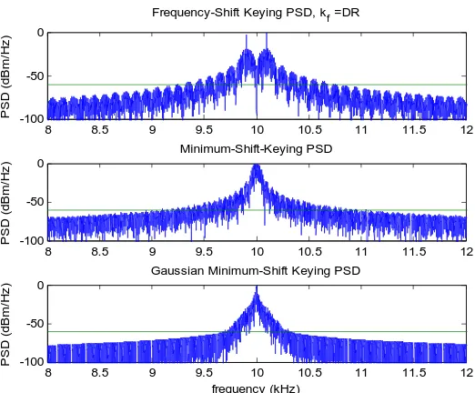
Figure 7 Comparison of several frequency-shift-keying modulation format spectra, showing decreased bandwidth.

Actually, a modified form of signaling called Gaussian FSK is more often used, for which the receiver design is easier. GFSK is used widely for portable wireless, in applications ranging from GSM cellular telephones to the Bluetooth wireless standard. GSM signaling uses a value of WT = 0.3 while Bluetooth signaling uses a value of WT=0.5.

7.2.4 Signal Constellation Modeling

It is sometimes difficult to visualize these waveforms, but an alternate means of

visualizing the signaling is available. These signal constellations provide the information necessary to understand both how the signals are produced and how the modulation scheme will perform in terms of BER.

Consider the QPSK waveforms based on rectangular pulse linecodes. In each of these modulation formats, we can regard the transmitted signal as a narrowband signal as modeled previously:

( )

( ) ( )

( ) ( )

( )

{

}

QPSK I c Q c

j t j t

g t x t t x t

A t e θ e ω

t

ω ω

= −

= . (7-7)

in-phase component, and xQ is the quadrature component. Define the complex envelope of the signal gQPSK(t) as

( )

( )

( )

( )

I Q

g t =g t +g t = A t eθ . (7-8)

Thus, the complex envelope of the carrier has a real part gI(t) and an imaginary part gQ(t). For the case of QPSK modulation, gI and gQ are both polar linecodes with rectangular pulses having some amplitude A during the symbol period.

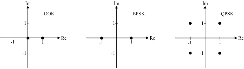
A signal constellation displays all possible vales of the complex envelope phasor. The signal constellations of OOK, BPSK, and QPSK are shown in Figure 8. For the case of OOK, only the cosine carrier component is used, and the gI component takes on only the values 0 and 1. BPSK also involves the modulation only of the cosine component, but the message values are +1 and -1, which give the phase shift.

In QPSK, both the cosine and sine carrier components are modulated, and thus the entire complex plane of the signal constellation must be used to represent the carrier envelope. Both the gI and gQ components are polar linecodes, so the 4 possible values for the complex envelope are: (Re,Im) = { (1,1), (1,-1),(-1,1),(-1,-1)}, as indicated in the constellation. Of course, an algorithm associating bit pairing (b0,b1) with points in the constellation must be specified, as this is not unique.

Re Im

OOK

Re Im

BPSK

Re Im

QPSK 1

-1 -1

1

1

-1 -1

1

1

-1 -1

1

Figure 8 Signal constellations for common digital modulation formats.

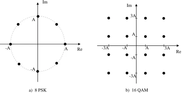
In general, there are two major classes of multilevel digital signaling, grouped by properties of the complex envelope and the form of the signal constellation produced. In Phase-Shift-Keying (PSK), the key differentiator is that the complex envelope has a constant magnitude – the data is encoded in the phase of the carrier only. This results in the signal constellation consisting of points lying on a circle. Note that the BPSK and QPSK signal constellations of Figure 8 fit this description.

Re Im

a) 8 PSK A

-A

-A

A

Re Im

b) 16 QAM -A

-3A

-3A

A 3A

-A A 3A

Figure 9 Example of signal constellations for a) MPSK for M=8, and b) M-symbol QAM for M=16.

Ultimately, the detection capability is an SNR problem. In the PSK case, the problem is one of phase discrimination. In some cases, however, simple amplitude discrimination can be performed to achieve detection.

In Quadrature Amplitude Modulation (QAM), the data is encoded in both the amplitude and phase of the complex envelope of the carrier. An example, 16-QAM, is shown in Figure 9b. For 16-QAM, four bits are encoded into each symbol. Specifically, two bits are encoded into a symbol pulse modulating the cosine component, and two bits are encoded into a symbol pulse modulating the sine component of the carrier.

Note that these m-ary signals are transmitted at a single carrier frequency, and have a double-sided bandwidth equal to the twice the baseband message bandwidth entering the modulation operation (that is, the symbol waveform modulating the carrier components). By combining multilevel signaling, pulse shaping, and IQ modulation, very efficient use of transmission bandwidth is achieved relative to the simple DSB-SC format.

The power spectral density for PSK or QAM signaling follows a standard sinc2 shape for the case of rectangular symbol pulses. If the number of points in the signal constellation is M=2q, then the null-to-null transmission bandwidth of PSK or QAM signal is 2*DR/q., where DR is the input bit rate. Note that the use of multilevel signaling thus explicitly reduces the transmission bandwidth as expected.

-1 0 1 -1.5

-1 -0.5 0 0.5 1 1.5

signal constellation w/o noise

I (V)

Q (

V

)

-1 0 1 -1.5

-1 -0.5 0 0.5 1 1.5

signal constellation w/ 20 dB SNR

I (V)

Q (

V

)

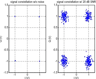
Figure 10 Signal constellation showing QPSK result with 20 dB CNR noise added.

The signal constellation allows the analyst to quickly gage the severity of the noise and its impact to BER. The signal constellation gives a relative measure of signal distance and noise variance visually presented. Small signal distance would be demonstrated as having the points of the constellation being placed close to one another in the absence of noise. Large noise variance is demonstrated by a wide variance of the points splattered around the expected value of the constellation point. These two values together reveal both SNR and BER information. Communication test equipment often has the ability to derive signal constellation diagrams built in to its software for quick examination of performance.

7.3 Choice of signaling format in system implementation

This chapter has presented many forms of digital modulation and several means of analyzing them. How does the system engineer go about choosing a modulation format, or understanding how a choice was made? First, it must be stressed that the decision is made based on inputs from the link design team based on requirements flowed down from the communication system engineers above. Second, only by considering many issues, most notably spectrum, data transmission quality, and throughput, can the choice be best understood. This section presents several of the major comparison categories by which the modulation formats are judged.

7.3.1 Performance comparison of digital modulation formats

predecessor. There are normally very good reasons why the incumbent format has been chosen, and this chapter has attempted to point out some of those reasons. A summary of some of the applications which have been associated with the various formats introduced in this chapter is given in Figure 11.

Figure 11 Examples of applications using the various digital modulation formats discussed.

However, at times a new modulation choice is warranted, and at that point it is important to be able to compare the various modulation choices available and suggest alternatives. To do this, there needs to be objective means to compare the performance of the various formats.

The performance measures we will be most interested in concern spectrum, data transmission quality and throughput. The first measure will be BER performance as a function of SNR or received power, which will have direct impact to the link budget. The second performance measure will be transmission spectrum. The third performance measure of interest will be a measure of data throughput per unit transmission bandwidth called the spectral efficiency. A final performance measure has to do with a practical implementation issue of amplifier nonlinearity.

7.3.1.1 Bit Error Rate Performance

that of a “waterfall”, with error probability falling sharply with increasing SNR. Noise, intersymbol interference and implementation loss in the receiver all reduce performance from the ideal curve practical implementations.

Similar conclusions hold for bandpass, symbol-based digital communication links. For bandpass modulation formats, the analysis of BER performance is most easily understood by changing the matched filter followed by a decision and sampling circuit to a correlator followed by the same decision and sampling circuit. This circuit can then operate either at baseband or for bandpass signaling. In either the baseband or the bandpass case, there is to be a decision made as to whether the signal is greater or less than a threshold, which leads to the Eb/N0 factor.

Binary modulation formats are easily compared with baseband polar signaling, from which their signaling is normally derived. Figure 12 shows such a comparison between common baseband and coherent bandpass signaling formats. (Non-coherent receiver performances suffer a slight performance degradation versus coherent, but the receivers are easier and cheaper to implement.)

1E-16 1E-14 1E-12 1E-10 1E-08 1E-06 0.0001 0.01 1

0 5 10 15 20

Eb/N0 (dB)

Pe

3 dB

ASK, FSK, Unipolar Baseband

BPSK, MSK, QPSK, and Polar Baseband

Figure 12 BER performance curve for binary modulation formats relative to baseband polar signaling.

Formats such as MSK and QPSK show advantage in that the receiver requires less power to achieve a given SNR. This required power to achieve a desired Pe (BER) is called the

Example: QPSK BER calculation

Example: Translate Eb/N0 to received power

7.3.1.2 Power Spectral Density and Bandwidth

One of the primary concerns to the digital communication system designer is bandwidth, and bandwidth has a meaning with several nuances. First, by bandwidth is meant the allowed (allocated) bandwidth given for your system to transmit its information. Your task, as system engineer, is to transmit information through that limited frequency band. Second, bandwidth describes the range of frequencies necessary to transmit the

information carrying modulated carrier. Different baseband linecodes, pulse shapes, and modulation formats all produce transmitted signals having different signal bandwidths. Finally, you must be a good citizen in the world of frequency allocation, and not interfere with your frequency (channel) neighbors. Therefore, there is a bandwidth beyond which your signal energy may not appreciable interfere with adjacent channels. In order to understand these definitions, and to design the systems, the system engineer must be comfortable with the power spectral densities of the various signaling formats described above.

Analytic expressions for the complex envelope PSDs for various forms of digital modulation are given in Figure 13 [1]. In each case, the input bit stream consists of a data rate of DR=1/Tb bits per second (bps). For quadrature schemes, the serial data stream is demultiplexed into parallel I and Q bitstreams at half rate. The symbols are rectangular unless otherwise noted. Note that while the formats have comparable main-lobe bandwidths, the -60 dB bandwidths, which offer a description of ACI impact, are dramatically different.

Signaling Format Complex Envelope PSD

Null-Null Transmission Bandwidth, BT

-60 dB Null-Null Bandwidth (approximate)

OOK/BPSK P f_g( )=Ksinc2

( )

QPSK/OQPSK P fg( )=Ksinc2

(

)

MPSK/MQAM

(M=2q)

(

)

2

( ) sinc

g

P f =K qT fb 2/q*DR 20/q*DR

MSK

(

)

(

)

(

)

2

2 2

cos 2 ( )

1 4

b g

b T f

P f K

T f π =

−

_{1.5*DR 3.0*DR}

Figure 13 Comparison of bandwidths of several modulation formats.

For comparison, each of the corresponding PSDs are plotted in Figure 14 as a function of frequency scaled by data rate. For each of these PSDs, rectangular symbol pulses are used. Keep in mind that some formats are binary, others are m-ary, and so the

Figure 14 Comparison of complex envelope Power Spectral Densities of several modulation formats.

There are a number of important features to note from these plots. First, note the sinc2 shape of the spectra, which results from the rectangular symbol pulse shape. Second, the “transmission bandwidth” is twice the complex baseband first null bandwidth in typical use. Minimizing bandwidth for a given data rate throughput is often an objective for system design. The only way to reduce this “main lobe” bandwidth is to change the pulse shape.

Finally, sidelobe content has much to do with adjacent channel interference, and so those formats which have greatly reduced sidelobe power content are preferred. A reference line drawn at a level 60 dB down from the peak power level is provided to emphasize this point. If adjacent channels require greater than 60 dB isolation, then the PSD must be at least this far down by the edge of the allocated frequency band for the adjacent channels. It is apparent why MSK and GMSK are so popular in terms of small ACI. Even though MSK has a larger null-null bandwidth than QPSK, its ACI performance is much better. It is noted that while GMSK can greatly reduce the bandwidth concerns, ISI-induced BER impact must be avoided.

(

)

T

DR B

q α

= + . (7-9)

Actually, depending upon the severity of the bandwidth limitation and ACI constraints, QPSK and its variants prove to be quite capable in many circumstances. However, as data throughput requirements rise, the bandwidth control issue becomes dominant.

7.3.1.3 Spectral Efficiency

The prime reality of modern communication system design is fixed and limited channel bandwidth. Between legislated allocations, interference concerns, and practical

implementation details, all communication links operate within a limited bandwidth. As demand for services increase, system engineers must solve the problem of sending more data through that fixed and limited bandwidth.

The spectral efficiency of a transmission format is defined as the link data rate divided by the transmission bandwidth.

T DR

B

η= . (7-10)

By link data rate is meant the actual rate of bit transmission across the link, including link overhead, as opposed to the information data rate, which describes the rate of data passed through the link.

To correctly compare spectral efficiencies of different modulation formats, a definition of transmission bandwidth must be agreed upon. For example, the bandwidth could be defined as the 90% power bandwidth occupied by the signal. For rectangular pulse signals, this corresponds to the null-to-null bandwidth of the power spectral density.

Example: Compare the spectral efficiency of OOK with that of QPSK.

A throughput data rate of DR is assumed. The baseband signal is a polar NRZ line code representation of digital data. This message has a

baseband bandwidth of DR, or, if using a DSB-SC carrier modulation scheme, a transmission bandwidth of 2DR, assuming the message signal bandwidth is equal to the first null of the PSD.Thus, for OOK, the throughput is DR, and the bandwidth is 2DR. The spectral efficiency for OOK is

1

2 2

ASK T

DR DR

B DR

η = = =

⋅ .

This results in the transmission of a DSB-SC carrier modulated signal with bandwidth DR. Using the quadrature multiplexer, we have achieved a transmission bandwidth reduction factor of 2 while maintaining the same throughput! The bit rate being transmitted is DR bps. Using the QPSK scheme, the spectral efficiency is increased to

1

QPSK T

DR DR

B DR

η = = = .

We would say that QPSK has twice the spectral efficiency of ASK. Of course, as the spectral efficiency increases, the difficulty in demodulating and detecting the signal increases, and not linearly!

In general, using M-ary signaling with rectangular pulse shaping, the spectral efficiency would be expected to scale as the log2M. Specifically,

2 2

M ary

DR q

DR q

η ₋ = =

⋅ . (7-11)

The spectral efficiency calculation should be examined carefully, and the same means of determining signal bandwidth applied to every situation evaluated. These efficiencies can be increased even further using pulse shaping techniques, such as implementing raised-cosine pulses.

7.3.1.4 Power Amplifier Nonlinearity Impacts

All amplifiers are linear only within a range of input signal amplitudes. The range of input single powers over which the amplifier is considered linear is described by the amplifier dynamic range. There are various types of amplifier designs, based in part upon their power efficiency and linearity. For example, Class C amplifiers, which offer good efficiency for portable wireless products, have issues with nonlinearity not found with other amplifier types.

The best signal design for use with Class C amplifiers is one which has a constant envelope (amplitude), which omits several of the basic modulation schemes discussed. We have found, for example, that the rectangular pulse QPSK family and MSK are constant envelope modulation formats, and so should operate well with power efficient Class C amplifiers in the handset transmitter. However, we also found that pulse shaping was desirable to reduce the sidelobe content for these signals. Pulse shaping introduces amplitude fluctuations in the envelope of the signal, although not as severe as rectangular pulse shaping.

Example: Simulate GMSK, OQPSK, OOK through simple nonlinearity

7.4 Summary

This chapter has presented many of the popular digital modulation formats available for modern link design. It turns out that many types of links today are built upon the versatile quadrature multiplexer/demultiplexer architecture, which supports the non-FSK digital modulation formats. The FSK formats are popular, especially teamed with Gaussian pulse shaping and incoherent receivers.

The system engineer is able to understand the behavior of the modulation formats in the time and frequency domains by studying their models and typical implementations. Often, these formats are simulated in model links to predict the actual performance according to the metrics described here and others that may be of interest.

7.5 References

1. Couch, L.W., Digital and Analog Communication Systems, 6th ed., 2001, Prentice-Hall.

2. Haykin, S. and Moher, M., Modern Wireless Communications, Pearson Prentice-Hall, 2005.