Optimal imaging with adaptive mesh refinement in electrical tomography

Physiol. Meas.23(2002) 121–128 PII: S0967-3334(02)30423-4

Optimal imaging with adaptive mesh refinement in

electrical impedance tomography

Marc Molinari1, Barry H Blott2, Simon J Cox1and Geoffrey J Daniell2

1_{Department of Electronics and Computer Science, University of Southampton, Southampton,}

SO17 1BJ, UK

2_{Department of Physics and Astronomy, University of Southampton, Southampton, SO17 1BJ,}

UK

E-mail: [email protected]

Received 13 July 2001, in final form 10 October 2001 Published 28 January 2002

Online atstacks.iop.org/PM/23/121

Abstract

In non-linear electrical impedance tomography the goodness of fit of the trial images is assessed by the well-established statisticalχ2_{criterion applied to the} measured and predicted datasets. Further selection from the range of images that fit the data is effected by imposing an explicit constraint on the form of the image, such as the minimization of the image gradients. In particular, the logarithm of the image gradients is chosen so that conductive and resistive deviations are treated in the same way. In this paper we introduce the idea of adaptive mesh refinement to the 2D problem so that the local scale of the mesh is always matched to the scale of the image structures. This improves the reconstruction resolution so that the image constraint adopted dominates and is not perturbed by the mesh discretization. The avoidance of unnecessary mesh elements optimizes the speed of reconstruction without degrading the resulting images. Starting with a mesh scale length of the order of the electrode separation it is shown that, for data obtained at presently achievable signal-to-noise ratios of 60 to 80 dB, one or two refinement stages are sufficient to generate high quality images.

Keywords: electrical impedance tomography, optimal imaging, image smoothness constraint, adaptive mesh refinement, reconstruction algorithm

(Some figures in this article are in colour only in the electronic version)

1. Introduction

Over the past three decades, much research has been carried out in the area of direct and inverse electric field problems (Geselowitz 1971, Webster 1990). Electrical impedance tomography (EIT) which measures the internal electrical property distribution has become a very active

research topic for medical applications. Some advantages of EIT over other imaging methods such as MRI or x-ray imaging are that it is very cost-effective, fast and portable but a key advantage is the close correlation of conductivity changes with the physiological function.

The finite element mesh is the accepted method of image representation in contemporary EIT. The speed of reconstruction and the resolution are competing factors in the choice of finite elements; large elements reduce computational time at the expense of resolution. However, resolution can be regained where it is necessary by adaptively adjusting the size of the elements as the image is reconstructed.

In this paper, we apply adaptive mesh refinement to non-linear EIT reconstruction and give examples of how this improves the image resolution while keeping the computational costs down. But first, we review the essential processes for generating well-characterized images in EIT; theχ2-statistic for goodness of fit is applied in conjunction with an explicit smoothness constraint on the image.

2. Review of imaging process

The problem of reconstructing a scalar conductivity distributionσwithin a bodyBconsists of solving the non-linear equation

∇ ·σ∇U =0 (1)

forσ. Here,Udenotes the potential at a point withinBresulting from a current injection normal to the surface of B. We denote the measured potentials at surface electrodes asVobserved₌

U(electrodes) and the electrode potentials based on the computed conductivity distributionσ asVpredicted_.

A conductivity distribution satisfying the equality of observed and predicted voltages is our target solution. However, all physical measurement processes have an inherent limitation in accuracy caused by the random noise generated in the signal source. The irreducible random noise contributionδV to the signalVobserved_{introduces statistical uncertainty in the imaging} process. The goodness of fit is then measured by theχ2_{-statistic, defined as}

χ2₌ M

i

Vpredicted

i −Viobserved δVi

2

. (2)

The criterion for an adequate fit is χ2 _{≈ M, where M is the number of independent} measurements. Values ofχ2_{Mwould suggest significant statistical disagreement between} Vpredicted_andVobserved_whileχ2 _{Mwould introduce artefacts intoσ solely to fit the noise} in the data. Even when an aqeduate fit is achieved a wide variety of solutions is possible. Because of the inherently limited spatial resolution of EIT, the values ofVpredictedare unaffected by small spatial scale fluctuations in conductivity, even of large amplitude. Hence solutions containing these still fit the data according toχ2and a means to restrict the range of solutions needs to be found.

One possible method to accomplish this is to construct an explicit measure of image quality, such as smoothness. Blottet al(1998a) chose a logarithmic function as the image constraint. It treats deviations in conductivity or resistivity in the same way and uses the local conductivity gradient as a definition of smoothness:

=

image|∇

logσ|2dxdy. (3)

We construct the following functional which we minimize with respect to the conductivityσ:

Start

Make initial uniform σ guess

Determine forward solution

Compute objective function Φ

End

Update σ by ∆σ

χ2_{≈ Μ ?}

yes no

refstep = max_refstep ? yes

no

Compute σ gradients Refine the mesh locally

refstep = refstep+1

χ2 _{converged ?} no

yes

Adjust λ

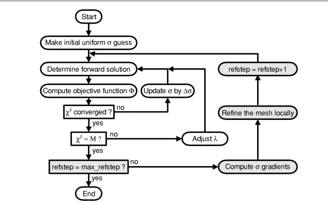
Figure 1. The modified iterative reconstruction algorithm incorporating material gradient estimation and auto-adaptive mesh refinement techniques. max refstep defines the maximal number of refinement steps allowed.

The parameterλis used as a weighting factor to balance between the contribution ofχ2_and the image smoothness function.λis adjusted untilχ2equalsMor cannot be reduced further. In the latter case, the noise level has been misjudged or systematic errors are present. One avoidable systematic error is discretizing the image space using a mesh that is too coarse so that the values ofVpredictedare not sufficiently accurate.

3. Adaptive mesh refinement

For the computational reconstruction the domain under investigation has to be discretized into small elements. We employ triangular finite elements with linear base functions and constant conductivity. If the pre-selected mesh is too coarse, the image resolution will be very poor. However, if the discretization is very fine, the search space for solutions is large and leads to a very slow reconstruction which may not even converge. We overcome this problem by using adaptive meshing. In the case of the forward problem—computing the potential distribution given the conductivities and injected current—we have shown (Molinariet al2001) that the finite element mesh need only be fine in regions where high current density gradients are present. These regions were identified by an error estimator constructed from current density residuals across inter-element boundaries.

is automatically refined in regions with high conductivity gradients. In order to apply (3) to a finite element representation ofσ(x, y) we need an approximation to . We use

edges

|log(σi)−log(σj)|2lij (5)

wherelijis the length of the edge separating elementsiandj. For deciding on whether to refine the mesh, we use the quantity|log(σi)−log(σj)|.

As a first approach, we refine elements whose average conductivity differences with its adjacent elements are larger than 40% of the maximal occurring difference in the mesh. This refinement criterion certainly needs adjustment as central elements exhibit a smoother transition than those closer to the boundary. In the test cases, this choice has always produced good results.

The selected elements are then refined by inserting vertices on the centres of all three edges. A local re-triangulation according to the Delaunay criterion (1934) is carried out and subsequent Laplacian mesh smoothing (Freitag 1997) ensures the use of near-equilateral elements (this is termed a ‘high quality’ mesh, see Molinariet alin this issue). This procedure is confined locally and is hence very fast. It is auto-adaptive in the sense that it does not require user interaction once the parameterλis chosen. Also, it is self-consistent in the sense that it does not require any prior information or knowledge about boundaries or approximate material distributions.

4. Simulation results

We have applied our algorithm (figure 1) to the reconstruction of data from several test structures. In this section we introduce a measure of image error, then present the reconstruction parameters and simulation results before investigating the effect of differing noise levels on the images.

4.1. Image comparison

To compare the reconstructed images with the simulated conductivity distributions we need a distance function as an indicator of reconstruction error. A direct method for comparing two images is to take the norm of the difference of conductivities at sample points across the image. Since we are comparing images reconstructed on triangular pixels, the simplest method to use would be to compare the material at the centre points of the finite elements. However, we are adapting and thus changing the underlying mesh including triangle sizes, shapes and positions so that this method is not applicable. In fact, some papers (e.g. Tanget al

2001) compare images on differing meshes using this method which could result in erroneous conclusions about the reconstruction accuracy achieved.

A better way of comparing images—which is also applicable to elements with higher order internal variation in conductivity—is to resample the image on a square grid which allows for comparison across a range of images. We define the distanceD between two conductivity images,σ1andσ2, by the application of the Frobenius norm as

D= 1

np np

i=1

(σ1(i)−σ2(i))2. ₍₆₎

0 0.5 1 0 0.2 0.4 0.6 0.8

1 a b c

d e f a b c d e f

0 0.5 1

0 0.2 0.4 0.6 0.8

1 a b c

d e f a b c d e f

0 0.5 1

0 0.2 0.4 0.6 0.8

1 a b c

d e f a b c d e f

0 0.5 1

0 0.2 0.4 0.6 0.8

1 a b c

d e f a b c d e f

(a) (b) (c) (d)

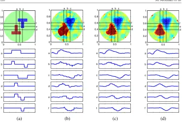
Figure 2. (a) Simulated conductivity distribution withσ=5 S m−1for lower T-shape andσ= 0.2 S m−1_{for upper T-shape. (b) Reconstruction at a SNR of 80 dB without mesh refinement,}

(c) after one refinement step, (d) after two refinement steps. The axes show the logarithmic conductivity corresponding to the cuts indicated in the image. The image is scanned from left to right and bottom to top at the slices indicated by lettersatof.

The normDcorresponds directly to the error of a reconstructed imageσ1=σreconif it is compared to the original simulated material distributionσ2=σsim. We will employ this quantity to obtain the absolute average errorEper pixel

E=D(σrecon, σsim). (7)

4.2. Reconstruction parameters

As an example we show the reconstruction of two T-shaped objects contained in a cylindrical area. The base conductivity of the cylinder is 1 S m−1_{and the conductivities of the objects} are 5 S m−1_{and 0.2 S m}−1_{respectively for lower and upper T. We investigate the resolution} at the centre as well as throughout the image by taking cuts through the object as indicated in figure 2(a) which shows the original conductivity distribution. The scale of the axes is logarithmic so that the conductivity values of the two objects are log (5) and log (0.2)=

−log (5) respectively, with the background conductivity set to log (1)=0. This example tests for image resolution at the centre and also for the symmetry in treatment of conductivity and resistivity deviations.

0 0.5 1 0 0.2 0.4 0.6 0.8

1 a b c

d e f a b c d e f

0 0.5 1

0 0.2 0.4 0.6 0.8

1 a b c

d e f a b c d e f

0 0.5 1

0 0.2 0.4 0.6 0.8

1 a b c

d e f a b c d e f

0 0.5 1

0 0.2 0.4 0.6 0.8

1 a b c

d e f a b c d e f

(a) (b) (c) (d)

Figure 3. (a) Simulated conductivity distribution withσ=5 S m−1for lower T-shape andσ= 0.2 S m−1_{for upper T-shape. (b) Reconstruction at a SNR of 60 dB without mesh refinement,}

(c) after one refinement step, (d) after two refinement steps. The axes show the logarithmic conductivity corresponding to the cuts indicated in the image.

14.1 s. We assume the hardware measurement of signal-to-noise ratio (SNR) to be in the range of 60 to 80 dB, which can be achieved with today’s measurement systems.

4.3. Results

Initial mesh elements are chosen with a scale to match the electrode spacing. Figure 2(b) shows the reconstruction on the initial coarse mesh with 304 elements after theχ2_{Mcondition has} been reached; this required four iteration steps. Applying one adaptive refinement step and iterating again results in the image in figure 2(c). We see clearly how the resolution even in the centre of the image has improved drastically. If we repeat this procedure again (figure 2d), further improvement is achieved; however, it is not as large as before if we compare the average pixel errorE.

Table1lists mesh sizes, error and reconstruction times at a noise level of 80 dB. The reconstructions were carried out in Matlab on a 900 MHz AMD-Athlon Processor with 1 GB RAM running the SuSE Linux 7.1 operating system.

The relatively large reconstruction time originates in the fact that the Newton–Raphson algorithm inverts a matrix of the size of the number of elements squared and in the computation of the smoothness constraint for each iteration. The inversion of the matrix could be avoided by the application of the so-called adjoint method (Arridge and Schweiger 1998) which does not require the explicit computation of the Jacobian in the reconstruction process.

4.4. Reconstructions at different noise level

(a)

(d)

(b) (c)

(f) (e)

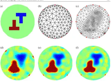
Figure 4. (a) Simulated conductivity distribution. (b) Initial mesh used for reconstruction. (c) Resulting mesh after three refinement steps during reconstruction. Reconstructions shown are at SNR’s of (d) 60 dB, (e) 80 dB and (f ) 170 dB.

Table 1. Reconstruction parameters before and after application of the adaptive reconstruction algorithm at a SNR of 80 dB.

Initial mesh After 1st refinement After 2nd refinement

Elements 304 533 1222

Nodes 201 316 663

ErrorE 0.008 0.005 0.004

Refinement (s) n.a. 1.10 2.22

Time/iteration (s) 0.59 1.26 5.31

Iterations required 4 4 4 (±1)

Total time for

reconstruction (s) 2.36 8.50 31.96

shown in table1; however, the error does not decrease as fast with increasing number of mesh refinements.

A third refinement results in no further improvements which means that the error is no longer sensitive to the discretization. This leads to the conclusion that the error is determined wholly by the smoothness constraint which in turn depends on the signal-to-noise ratio of the measurement system.

5. Discussion and conclusions

In this paper we have focused on the issue of unavoidable random noise as the ultimate factor governing the optimum quality of image attainable in EIT. We have shown that the application of adaptive mesh refinement allows for the effective operation of an explicit image constraint. The choice of constraint to generate optimal images will depend to some extent on the nature of the interpretations sought by the user. Here we have chosen to select the smoothest images consistent with fitting the data. The results demonstrate clearly that the degree of detail which may be imaged depends on the level of random noise in the data. With presently available systems, the level of signal-to-noise achievable with a few seconds of data is in the range of 60–80 dB. At these levels we have found that one or two refinement stages are sufficient to prevent the mesh discretization from affecting the image.

We have not considered the effect of systematic errors which may, in principle, be discoverable. The positions of the electrodes are measurable, but small movements during measurement may be unavoidable and their effect may need to be attenuated (Blottet al1998b). Systematic effects may appear as distortions in the images where account may be taken of them, or they may appear as an inability to minimizeχ2during the reconstruction process. In which case they may have to be included in the estimate of noise used to constructχ2.

However, we have demonstrated that it is not necessary to uniformly refine the mesh to improve the solution quality, only to locally adapt where the reconstruction algorithm indicates large gradients in conductivity. This has a clear benefit in the computation time required whilst not sacrificing essential accuracy. The advantages of tuning the element density adaptively at solution time are even greater in 3D EIT (Molinariet al2002).

Acknowledgment

MM is grateful to EPSRC for financial support.

References

Arridge S and Schweiger M 1998 A gradient-based optimisation scheme for optical tomographyOptics Express2

213–26

Blott B H, Daniell G J and Meeson S 1998a Nonlinear reconstruction constrained by image properties in electrical impedance tomographyPhys. Med. Biol.431215–24

Blott B H, Daniell G J and Meeson S 1998b Electrical impedance tomography with compensation for electrode positioning variationsPhys. Med. Biol.431731–9

Delaunay B N 1934 Sur la SphereVide. Izvestia Akademia Nauk SSSR, VII Seria, Otdelenie Matematicheskii i Estestvennyka Nauk7793–800

Freitag L A 1997 On combining laplacian and optimization-based mesh smoothing techniquesAMD-Vol. 220 Trends in Unstructured Mesh Generation, ASME(July 1997) pp 37–43

Geselowitz D B 1971 An application of electrocardiographic lead theory to impedance plethysmographyIEEE. Trans. Biomed. Eng.1838–41

Isaacson D 1986 Distinguishability of conductivities by electric current computed tomographyIEEE Trans. Med. Imaging591–5

Molinari M, Cox S J, Blott B H and Daniell G J 2001 Adaptive mesh refinement techniques for electrical impedance tomographyPhysiol. Meas.2291–6

Molinari M, Cox S J, Blott B H and Daniell G J 2002 Comparison of algorithms for non-linear inverse 3D electrical tomography reconstructionPhysiol. Meas.2395–104

Tang M, Wang W and Wheeler J 2001 Incorporating more compatible prior information into the image in electrical impedance tomographyThird EPSRC Engineering Network Meeting on Biomedical Applications of EIT— Scientific Abstracts(University College London, UK, April 4–6 2001) pp 37–40