Block Adaptive Kernel Based CDMA Multiuser Detector

Block-Adaptive Kernel-Based CDMA Multiuser Detection

Department of Electronics and Computer Science University of Southampton, Southampton SO17 1BJ, U.K.

Abstract— The paper investigates the application of a recently intro-duced learning technique, referred to as the relevance vector machine (RVM) to construct a block-adaptive kernel-based nonlinear multiuser detector (MUD) for direct-sequence code-division multiple-access (DS-CDMA) signals transmitted through multipath channels. It is demon-strated that the RVM MUD is capable of closely matching the perfor-mance of the optimal Bayesian one-shot detector, with the aid of a sig-nificantly more sparse kernel representation than that required by the state-of-the-art support vector machine (SVM) technique.

I. INTRODUCTION

Although the linear minimum mean square error (MMSE) MUD [1]–[5] is widely used for DS-CDMA downlink systems due to its simplicity, its limitation has long been recognized – a linear detec-tor results in a residual bit error ratio (BER), unless the underly-ing noise-free signal classes are linearly separable. However, since linearly non-separable cases are common in DS-CDMA channels, often a better performance can be obtained by using a nonlinear MUD. Hence neural networks [6] have been considered as nonlin-ear MUDs [7]–[10]. However, the training period required by these nonlinear MUDs may become excessive and/or unpredictable. Fur-thermore, the structure of these neural network aided MUDs is often

ad hoc.

In our previous work [11],[12] the SVM technique [13]–[15] has been applied for constructing kernel-based MUDs. Our study has shown that an SVM aided MUD trained using a relatively small block of noisy received signal samples may closely approximate the performance of the optimal MUD, although the latter requires a complete knowledge of the system, namely that of the system ma-trixPand the noise variance. Another advantage of the SVM ap-proach over the existing nonlinear MUDs is the direct definition of the detector’s structure, which is specified by a sparse set of support vectors (SVs) selected automatically from the data during the learn-ing process. However, as the results reported in [11],[12] show, when applied to the MUD problem, the SVM technique does not produce a sufficiently sparse model in the sense that a typical SVM aided MUD will have 2 to 8 times more kernels, than the number of the noise-free signal states that is required by the optimum Bayesian detector.

Recently, Tipping [16] introduced a RVM method, which is based on a Bayesian framework [17],[18] and has an identical functional form to that of the SVM. The results given in [16] have demon-strated that the RVM has a comparable generalization performance to that of the SVM, while requiring significantly less kernel func-tions than the SVM. This paper investigates the application of the RVM technique to the construction of a block-adaptive kernel-based MUD. The computer simulation results confirm that the RVM as-sisted MUD is capable of closely matching the optimal Bayesian

performance, and it exhibits a significantly sparser kernel represen-tation than the SVM aided MUD. More specifically, an RVM as-sisted MUD typically has fewer kernels functions, than the number of noise-free signal states. That is, it can be typically described with the aid of a sparser representation, than the optimal Bayesian detector. The main drawback of the RVM method is, however that it involves a highly nonlinear optimization process. Hence the RVM assisted MUD’s performance has to be compared to that of the SVM technique, which is required to solve a significantly simpler quadratic problem.

II. SYSTEM MODEL

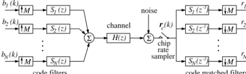
The discrete-time model of the synchronous downlink DS-CDMA system supportingN users and transmittingM (> N) chips per bit is depicted in Fig. 1, wherebi(k)∈ {±1}denotes thek-th bit of useri. Furthermore, the unit-length signature code sequence of useriis¯si = [¯si,1· · ·¯si,M]T, and the z-domain transfer function associated with the channel impulse response (CIR) is given by:

H(z) = nh−1

X

i=0

hiz−i. (1)

The bit vector ofNusers at instantkisb(k) = [b1(k)· · ·bN(k)]T, and the received signal vector after the chip-matched filters is r(k) = [r1(k)· · ·rN(k)]T. It can be shown that the baseband model forr(k)is:

r(k) =P 

  

b(k)

b(k−1)

.. . b(k−L+ 1)



  

+ ˜n(k), (2)

where theN_×LNsystem matrix is given by

P= ¯STH 

   

¯

SU 0 _{· · ·} 0

0 SU¯ . .. ... ..

. . .. . .. 0 0 _{· · ·} 0 SU¯



   

; (3)

the user signature sequence matrix isS¯= [¯s1· · ·¯sN]; the diagonal user signal amplitude matrix isU = diag{U1· · ·UN}; theM×

LMCIR matrixHhas the form of:

H=



  

h0 h1 _{· · ·} hnh−1

h0 h1 · · · hnh−1

. ._. . ._{. · · ·} . ._.

h0 h1 · · · hnh−1



  

;

..

.

.

..

b (k)

b (k)

b (k) 1

S (z)

S (z) 1

2 M

M

M

M

M

M S (z )

S (z )

S (z ) 1

2 Σ

r (k)

r (k)

S (z)N N

H(z) channel

noise

code matched filters Σ

2

N

1

2

N -1

-1 -1

code filters

chip rate sampler

r (k)

(k) r_c

Fig. 1. Discrete-time model of the synchronous CDMA downlink.

and orthogonal code sequences are assumed, so that the noise vector n˜(k) = [˜n1(k)· · ·n˜N(k)]T at the outputs of the chip-matched filters n˜(k) = [˜n1(k)· · ·n˜N(k)]T has a covariance of

E[˜n(k)˜nT_{(k)] =σ}2

nI. We note that the orthogonality of the codes is destroyed by the channel-induced intersymbol interference (ISI). The ISI spanLdepends on the lengthnhof the CIR, expressed in terms of the number of chipsM per spreding code. Fornh = 1 we haveL = 1; for1< nh ≤M,L= 2; forM < nh ≤2M,

L= 3; and so on.

III. LINEAR AND OPTIMAL DETECTORS

The linear MUD of userihas the form:

ˆ_{bi(k) = sgn(yL(k)) with yL(k) =w}T

r(k), (5)

wherew = [w1· · ·wN]Tdenotes the MUD’s weight vector. The most popular solution for the MUD of (5) is the MMSE solution given by

wM M SE= σn2I+PPT

−1

pi, (6)

wherepidenotes thei-th column ofP. The linear MUD of (5) has a low computational complexity, and the standard LMS or RLS algorithms can be used for implementing the MMSE solution adap-tively.

However, a linear MUD only performs adequately in certain situa-tions. Let theNb= 2LN possible combinations of[bT(k)bT(k− 1)· · ·bT(k−L+ 1)]T

be

b(j)=



   

b(j)_(k) b(j)(k−1)

.. . b(j)_(k

−L+ 1)



   

,1≤j≤Nb, (7)

andb(_ij) be theith element ofb(j)(k). Let us furthermore define the set of theNbnoise-free received signal states as:

R={rj=Pb(j), 1≤j≤Nb}. (8)

In case of ninary transmissionRcan be partitioned into two subsets:

R±={rj∈ R:bi(j)=±1}. (9)

IfR−andR+are not linearly separable, a linear MUD will have an irreducible error floor even in the noise-free case, as it can only form a decision hyperplane in theN-dimensional received signal space. It was demomstrated with the aid of an example in [6] that

this error floor can be potentially removed, if the decisions are cast into a higher-dimensional space.

Applying the maximum a posteriori probability (MAP) or Bayesian classification theory in a manner similar to the channel equalization problem [19], it can be shown that the optimal detector has the form:

yB(k) = Nb

X

j=1

βjb(ij)exp

−kr(k)−rjk

2

2σ2

n

(10)

with

ˆ_{bi(k) = sgn(yB(k)), (11)}

whereb(_ij)∈ {±1}serve as class labels, and all the channel states are assumed to be equiprobable withβj= 1

Nb(2πσ2n) m

2 .

IV. THE RELEVANCE VECTOR MACHINE DETECTOR

The optimal detector of (10) requires the knowledge of all the noise-free signal satesrj, which are unknown to receiveri. In general, the receiver can have access to a block ofKtraining samples{xk =

r(k), tk=bi(k)}Kk=1. Consider the kernel-based detector of useri in the form of:

y(r(k)) = K

X

l=1

wlFl(r(k)), (12)

wherewlare the “weights” andFl(r(k)) =F(r(k),xl). Observe that instead of theN-dimensional weight vector of the linear de-tector of 5, here aK-dimensional weight-vector is used. For this application, the kernel functionF(·,·)is naturally chosen to be a Gaussian function, with its variance being an estimate of the chan-nel’s noise variance. The relevance vector (RV) approach of clas-sification [16] can readily be applied for constructing the detector (12). Denote theK-dimensional vector of previously defined train-ing samples{xk=r(k), tk=bi(k)}Kk=1byt= [t1· · ·tK]T and the weight vector byw= [w1_{· · ·}wK]T. The posterior probability ofwis

p(w_|t,α) = p(t|w,α)p(w|α) p(t|α)

, (13)

wherep(w_|α)is the a priori probability of the weight vectorw conditioned onα = [α1· · ·αK]T denoting the vector of hyper-parameters, which is a term well established in statistical decision theory [17],p(t|w,α)is the so-called likelihood [17] andp(t|α) the evidence [17]. Following the Bayesian classification framework [18], the likelihood can be expressed as

p(t_|w,α) =

K

Y

l=1

(f(y(xl)))tl(1−f(y(xl)))1−tl, (14)

where

f(x) = 1

1 + exp(−x) (15)

is the logistic sigmoid function. The Gaussian a priori probability is chosen in the form of:

p(w_|α) =

K

Y

l=1

√

αl √

2πexp

−αlw

2

l 2

Since the so-called marginal likelihoodp(t|α)cannot be obtained analytically by integrating out the weights from (14), an iterative procedure is necessitated [18].

With a given fixedα, the MAP solutionwMAP can be obtained by maximizinglog(p(w_|t,α))or, equivalently, by minimizing the following cost function

J(w|t,α) =

K

X

l=1

{αlw

2

l

2 −tllog(f(y(xl)))

−(1−tl) log(1−f(y(xl)))}. (17)

The gradient ofJwith respect towis given by:

∇J=Aw+ΦT(f₋t), (18)

whereA = diag{α1,· · ·, αK}, f = [f(y(x1))· · ·f(y(xK))]T and the matrixΦhas elementsφi,j =F(xi,xj). The Hessian of

Jis

H=∇2J=ΦTBΦ+A, (19) whereB = diag{f(y(x1))(1−f(y(x1))),_{· · ·}, f(y(xK))(1−

f(y(xK)))}.

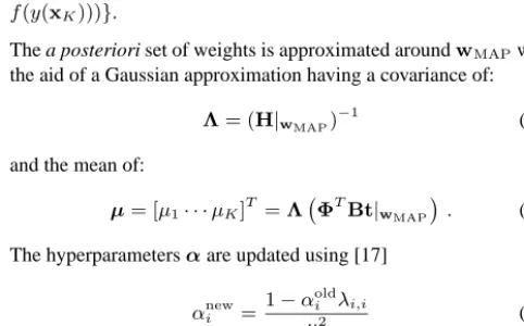
The a posteriori set of weights is approximated aroundwMAPwith the aid of a Gaussian approximation having a covariance of:

Λ= (H|w_MAP) −1

(20)

and the mean of:

µ= [µ1· · ·µK]T=Λ ΦTBt|w

MAP

. (21)

The hyperparametersαare updated using [17]

αnewi =

1−αoldi λi,i

µ2

i

(22)

withλi,ibeing the diagonal elements ofΛ.

The introduction of an individual hyperparameter for every weight of the model (12) is the key feature of the RVM aided approach, and it is ultimately responsible for its attractively low number of ker-nels [16]. During the optimization process, many of theαi hyper-parameters are driven to large values and hence the corresponding model weightswiare effectively pruned out. Thus the correspond-ing model termsFi(·)can be removed from the trained model rep-resented by (12). The simple iterative procedure that we adopt for constructing a RVM aided MUD is summarized as follows:

Initialization. TheK_×nRkernel matrixΦis initialized withnR=K, i.e. every training data point is considered as a candidate kernel. Each weightwiis initially associ-ated with an identical value of the hyperparameterαi.

Step 1. Given the current valueα, findwMAP by mini-mizing the cost function of (17). A simplified conjugate gradient algorithm [20] is used in the optimization. Al-ternatively, the iteratively-re-weighted least-square algo-rithm [21] can be used.

Step 2. The hyperparameters are updated using (22). If we

haveαi> Lg, whereLgis a preset large positive value,

we assignnR :=nR−1, and the corresponding column inΦis removed. Thus the corresponding weightwiand model termFi(·)is pruned out the model.

Test. If the hyperparametersαremain sufficiently un-changed in two successive iterations or a pre-set maxi-mum number of iterations is reached, stop; otherwise go to Step 1.

The set of RVs{xl}nl=1R selected is typically a small subset of the training points. The RVM aided MUD thus computes the decision variable as follows:

y(r(k)) = nR

X

l=1

wlFl(r(k)) (23)

and carries out the decision according to:

ˆ_{bi(k) = sgn(y(r(k))). (24)}

V. SIMULATION RESULTS

Two simulation examples were used for comparing the performance of the proposed RVM aided MUD to that of the linear MMSE, opti-mal Bayesian and the SVM assisted MUDs. It is worth pointing out

again that the linear MMSE and the optimal MUDs are designed based on the complete knowledge of the system (the system matrix Pand the noise variance), while the SVM and RVM aided MUDs are trained using a block of the noisy received signal samples.

Example 1. This was a two-user system with 4 chips per bit.

The code sequences of the two users were(+1,+1,−1,−1)and

(+1,−1,−1,+1), respectively, and the transfer function associ-ated with the CIR wasH(z) = 0.3 + 0.7z−1+ 0.3z−2. The two users had equal signal power, that is, the signal to noise ratio SNR1 of user 1 was equal to SNR2 of user 2. In order to construct a kernel-based MUD for user 2, a total of 160 training data points were generated for each given noise variance. The number of SVs selected by the SVM method is influenced by the control parameter C, which provides a trade-off between the model’s complexity (the number of SVs) and the training error [13]. The appropriate value forC was found in the simulations experimentally. When using C= 8.0, the number of SVs was found typically to be around 40. For the RVM method, there was no need to specify such a control parameter, and the numbers of RVs found ranged from 6 (for low SNRs) to 18 (for high SNRs).

TABLE I

BERPERFORMANCE AND NUMBER OF KERNELS USED BY VARIOUS

MUDS FOR USER2OFEXAMPLE1,GIVENSNR1=SNR2= 20DB. THESVMUSEDC= 8.0.

model log10(BER) kernels

SVM -3.019 40

RVM -3.045 18

Bayesian -3.155 16

Example 2. This was a 3-user system employing 8

chips per bit. The code sequences for the three users were (+1,+1,+1,+1,₋1,₋1,₋1,₋1), (+1,₋1,+1,₋1,₋1,

+1,−1,+1) and (+1,−1,−1,+1,−1,+1,+1, −1), respec-tively, and the z-domain transfer function associated with the CIR wasH(z) = 0.5 + 1.0z−1−0.5z−2. The three users had equal signal power. The number of training data used for constructing the kernel-based MUDs was 640 for each given SNR. For user 3, typ-ically 200 SVs were selected from the training data set, while the number of RVs selected ranged from 14 (for low SNRs) to 38 (for high SNRs). Table II summarizes the results for three MUDs, given SNRi= 15dB,1≤i≤3. The BERs of the resultant RVM aided MUDs of user 3 experienced under different SNR conditions are given in Fig. 4, in comparison to the corresponding linear MMSE and optimal MUDs. The results again demonstrate that the RVM aided MUD is capable of closely approximate the performance of the optimal detector using a low number of kernels. This reduces the complexity of classifying the received signal vector into one of the legitimate classes, which is ultimately required for carrying out a binary decision.

VI. CONCLUSIONS

The RVM technique has been applied for adaptive nonlinear mul-tiuser detection in DS-CDMA systems. It has been shown that the RVM MUD trained using noisy data is capable of closely approx-imating the performance of the optimal Bayesian one-shot detec-tor using less kernels than the Bayesian MUD. Compared to the SVM aided technique, the RVM assisted MUD results in a less com-plex received vector classification in the MUD. A disadvantage of the RVM aided MUD is, however that it requires solving a more complex nonlinear optimization problem. Like the SVM method, the RVM method is a block-based technique. Future research is required for investigating how to incorporate a sample-by-sample

TABLE II

BERPERFORMANCE AND NUMBER OF KERNELS USED BY VARIOUS

MUDS FOR USER3OFEXAMPLE2,GIVENSNRi= 15DB,1≤i≤3. THESVMUSEDC= 5.0.

model log₁₀(BER) kernels

SVM -2.452 199

RVM -2.489 30

Bayesian -2.780 64

-2 -1.5 -1 -0.5 0 0.5 1 1.5 2

-2 -1.5 -1 -0.5 0 0.5 1 1.5 2

r2(k)

r1(k)

b2(k) =−1

b2(k) = 1

+ + + + + + + + × × × × × × × × e e e e e e e e e e e e e e e e e e e e e e e e e e e e e e e e e e e e e e e e r r r r r rr r r r r r r r r r r r r r r r r r r r r r r r r r r r r r r r r r r r r r r r r r r r r r r r r r r r r r r r r r r r r r r r r r r r r r r r r b b b b b b b b b b b b b bb b b b b b b b b b b b b b b b b b b b bb b b b b b b b b b b b b b b b b b b b b b b b b b b b b b b b b b b b b b b b b b b b b b (a) -2 -1.5 -1 -0.5 0 0.5 1 1.5 2

-2 -1.5 -1 -0.5 0 0.5 1 1.5 2

r2(k)

r1(k)

b2(k) =−1 b2(k) = 1

+ + + + + + + + × × × × × × × × e e e e e e e e e e e e e e e e e e r r r r r rr r r r r r r r r r r r r r r r r r r r r r r r r r r r r r r r r r r r r r r r r r r r r r r r r r r r r r r r r r r r r r r r r r r r r r r r r b b b b b b b b b b b b b bb b b b b b b b b b b b b b b b b b b b bb b b b b b b b b b b b b b b b b b b b b b b b b b b b b b b b b b b b b b b b b b b b b b (b)

-5 -4 -3 -2 -1 0

4 8 12 16 20 24

log10(Bit Error Rate)

SNR2 (dB) linear MMSE

RVM Optimal

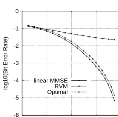
Fig. 3. Performance comparison of three MUDs, linear MMSE, adaptive RVM and optimal detectors, for user 2 of Example 1. SNR1=SNR2, and the training data set for RVM had 160 samples. The numbers of RVs found ranged from 6 (for low SNRs) to 18 (for high SNRs).

-6 -5 -4 -3 -2 -1 0

4 8 12 16 20

log10(Bit Error Rate)

SNR3 (dB) linear MMSE

RVM Optimal

Fig. 4. Performance comparison of three MUDs, linear MMSE, adaptive RVM and optimal detectors, for user 3 of Example 2. SNRi,1≤i ≤3,

were identical, and the training data set for RVM had 640 samples. The num-bers of RVs found ranged from 14 (for low SNRs) to 38 (for high SNRs).

adaptive methodology into the RVM approach.

REFERENCES

[1] Z. Xie, R.T. Short and C.K. Rushforth, “A family of suboptimum de-tectors for coherent multiuser communications,” IEEE J. Selected

Ar-eas in Communications, Vol.8, No.4, pp.683–690, 1990.

[2] U. Madhow and M.L. Honig, “MMSE interference suppression for direct-sequence spread-spectrum CDMA,” IEEE Trans.

Communica-tions, Vol.42, No.12, pp.3178–3188, 1994.

[3] S.L. Miller, “An adaptive direct-sequence code-division multiple-access receiver for multiuser interference rejection,” IEEE Trans.

Communications, Vol.43, No.2/3/4, pp. 1746–1755, 1995.

[4] H.V. Poor and S. Verd´u, “Probability of error in MMSE multiuser de-tection,” IEEE Trans. Information Theory, Vol.43, No.3, pp.858–871, 1997.

[5] G. Woodward and B.S. Vucetic, “Adaptive detection for DS-CDMA,”

Proc. IEEE, Vol.86, No.7, pp.1413–1434, 1998.

[6] L. Hanzo, C.H. Wong, M.S. Yee: Adaptive wireless transceivers: Turbo-Coded, Turbo-Equalised and Space-Time Coded TDMA, CDMA and OFDM systems, John Wiley, in press

[7] B. Aazhang, B.P. Paris and G.C. Orsak, “Neural networks for mul-tiuser detection in code-division multiple-access communications,”

IEEE Trans. Communications, Vol.40, No.7, pp.1212–1222, 1992.

[8] U. Mitra and H.V. Poor, “Neural network techniques for adaptive multiuser demodulation,” IEEE J. Selected Areas in Communications, Vol.12, No.9, pp.1460-1470, 1994.

[9] D.G.M. Cruickshank, “Radial basis function receivers for DS-CDMA,” Electronics Letters, Vol.32, No.3, pp.188-190, 1996. [10] R. Tanner and D.G.M. Cruickshank, “Volterra based receivers for

DS-CDMA,” in Proc. 8th IEEE Int. Symp. Personal, Indoor and Mobile

Radio Communications, September 1997, Vol.3, pp.1166-1170.

[11] S. Chen, A.K. Samingan and L. Hanzo, “Adaptive multiuser receiver using support vector machine technique,” Proceedings of VTC 2001

Spring Conf. (Rhodes, Greece), May 6-9 2001, pp 604-608

[12] S. Chen, A.K. Samingan and L. Hanzo, “Support vector machine mul-tiuser receiver for DS-CDMA signals in multipath channels,” IEEE

Trans. Neural Networks, Vol. 12, No.3, May 2001, pp 604-611

[13] V. Vapnik, The Nature of Statistical Learning Theory. New York: Springer-Verlag, 1995.

[14] B. Sch¨olkopf, K.K. Sung, C.J.C. Burges, F. Girosi, P. Niyogi, T. Pog-gio and V. Vapnik, “Comparing support vector machines with Gaus-sian kernels to radial basis function classifiers,” IEEE Trans. Signal

Processing, Vol.45, No.11, pp.2758–2765, 1997.

[15] C.J.C. Burges, “A tutorial on support vector machines for pattern recognition,” Data Mining and Knowledge Discovery, Vol.2, No.2, pp.121–167, 1998.

[16] M.E. Tipping, “The relevance vector machine,” in Sara A. Solla, Todd K. Leen and Klaus-Robert M ¨uller, eds., Advances in Neural

Informa-tion Processing Systems 12, Cambridge, MA: MIT Press, 2000.

[17] D.J.C. MacKay, “Bayesian interpolation,” Neural Computation, Vol.4, No.3, pp.415–447, 1992.

[18] D.J.C. MacKay, “The evidence framework applied to classification networks,” Neural Computation, Vol.4, pp.720–736, 1992.

[19] S. Chen, B. Mulgrew and P.M. Grant, “A clustering technique for dig-ital communications channel equalisation using radial basis function networks,” IEEE Trans. Neural Networks, Vol.4, No.4, pp.570–579, 1993.

[20] M.S. Bazaraa, H.D. Sherali and C.M. Shetty, Nonlinear Programming:

Theory and Algorithms. New York: John Wiley, 1993.

[21] I.T. Nabney, “Efficient training of RBF networks for classification,” in