Abstract— Machining or metal cutting is one of the most widely used production processes in industry. The quality of the process and the resulting machined product depends on parameters like tool geometry, material, and cutting conditions. However, the relationships of these parameters to the cutting process are often based mostly on empirical knowledge. In this study, computer modeling and simulation using LS-DYNA software and a Smoothed Particle Hydrodynamic (SPH) methodology, was performed on the orthogonal metal cutting process to analyze three-dimensional deformation of AISI 1045 medium carbon steel during machining. The simulation was performed using the following constitutive models: the Power Law model, the Johnson-Cook model, and the Zerilli-Armstrong models (Z-A). The outcomes were compared against the simulated results obtained by Cenk-Kiliçaslan using the Finite Element Method (FEM) and the empirical results of Jaspers and Filice. The analysis shows that the SPH method combined with the Zerilli-Armstrong constitutive model is a viable alternative to simulating the metal cutting process. The tangential force was overestimated by 7% and the normal force was underestimated by 16% when compared with empirical values. The simulation values for flow stress versus strain at various temperatures were also validated against empirical values. Experimental work was also done to investigate the effects of friction, rake angle and tool tip radius on the simulation..
Index Terms— Metal Cutting Simulation, Smoothed Particle Hydrodynamics, Constitutive Models, Cutting Forces Analyses
I. INTRODUCTION
ACHINING or metal cutting is one of the most widely used production processes in industries. The process allows the creation of parts with complex geometries, dimensional accuracy and fine tolerances. The quality of the process and the resulting machined product depends on parameters like tool geometry, material, and cutting conditions. However, the relationships of these parameters to the cutting process are often based only on empirical knowledge. Experimental investigations to study metal cutting processes are time consuming and expensive. Despite the availability of machining databases of these experimental approaches, the development of new materials,
Manuscript received March 20, 2017; revised April 06, 2017.
Seyed Hamed Hashemi Sohi is with the Mechanical Engineering Department, University of the Philippines Diliman, Quezon City, Metro Manila, Philippines (phone: +63-927-1553815; e-mail: [email protected]).
Gerald Jo C. Denoga is with the Mechanical Engineering Department, University of the Philippines Diliman, Quezon City, Metro Manila, Philippines (e-mail: [email protected]).
tools and machines have made these databases unreliable and irrelevant. Hence, alternative methods of analyzing the cutting process are needed in order to specify the process parameters and selecting the best tools for each process.
Computer simulation using the Finite Element Method (FEM) is a popular alternative approach. However, FEM is implemented using either of the following approaches: Lagrangian, Eulerian, Arbitrary Lagrangian-Eulerian, and Smoothed Particle Hydrodynamic. Unfortunately, the first three finite element methods entail the creation of meshes that cannot handle big deformations that occur with the metal cutting process. In contrast, the Smoothed Particle Hydrodynamic (SPH) method solves this issue by being a mesh-free method, eliminating element distortion during the simulation of the machining process. This method has improved during last decade which is mostly used in fluid and continuum mechanics and recently developed for solid mechanics problem. Researchers like Limido et al. [4]. Morten et al. [5] and Bagci[6] simulated the metal cutting process with the SPH method on aluminum and die steel; all of them mentioned that its features are not fully understood, and the most effective means to exploit it are still being discovered.
In this study, modeling and simulation of orthogonal metal cutting is performed on AISI 1045 material from the viewpoint of force analysis of three-dimensional deformation using SPH methodology through different constitutive models via LS-DYNA software, by comparing the outcomes with the results that have been obtained by CenkKiliçaslan [1] with FEM method and empirical results of Jasper [2] and Filice et. al [3].
Due to the fact of the newness of the SPH method in simulation of metal cutting, its features and performances are not completely understood. Consequently, there were some limitations to conduct the research in part of comparison of the results with the empirical ones such as stresses and different force values, but this method has been seen very reliable and can develop to new field of metal cutting simulations.
II. MATHEMATICAL MODEL A. Smoothed Particle Hydrodynamic method
The Smoothed Particle Hydrodynamic technique involves the use of kernel approximation and particle approximation formulations. The kernel approximation of a function is done by integrating the product of the derivative of the function and a smoothing function, as shown in the formula below:
Orthogonal Metal Cutting Simulation of Steel
AISI 1045 via Smoothed Particle
Hydrodynamic Method
Seyed Hamed H. Sohi and Gerald Jo C. Denoga
〈𝑓(𝑥)〉 = ∫ ƒ(𝑥′)𝑊(𝑥 − 𝑥′, ℎ) 𝛺
𝑑𝑥′ (1)
Where (ℎ) is the smoothing length, defining the influence or support area of the smoothing function (𝑊) in the problem domain (𝛺). In this formulation, the influence area of interacting particles in the continuum represented by smoothing length is usually assumed to be 2 ℎ distance and the interaction weighted by the kernel function 𝑊. Lacome [20], uses the smoothing kernel function below:
𝑊(𝑥𝑖− 𝑥𝑗, ℎ̅) = 1
ℎ 𝜃 (
𝑥𝑖− 𝑥𝑗
ℎ̅ ) (2)
The ideal smoothing length is achieved when the particles considered in the domain are enough to validate the particle approximations of the continuum variables. The option of a variable smoothing length is the default in LS-DYNA [20]. The time rate of change for smoothing length is given by the following equation:
𝑑ℎ
𝑑𝑡 =
1
3ℎ̅𝛻. 𝑉 (3)
Particle approximation represented by Lacome [7-8], Lacome et al. [9] and Ls-Dyna theoretical manual Hallquist [11] to change the weight and movement of the set of particles in domain (𝛺) formulated as below:
∇𝑆ℎ(𝑥
𝑖) = ∑ 𝑚𝑗
𝑆(𝑥𝑗)
𝜌(𝑥𝑗)
𝑁
𝑗=1
𝛻𝑤(𝑥𝑖− 𝑥𝑗, ℎ̅) (4)
Which applies a gradient operator to the smooth particle approximation
𝑆
ℎ(𝑥
𝑖).
A. Power Law material model
The model that Oxley [10] and his co-workers
represented for material flow stress of carbon steels by use the Power law is defined below:
𝜎 = 𝐾𝜀𝑛[1 + (𝜀̇
𝐶)
𝑝
] (7)
Where σ and 𝜀 are flow stress and strain, 𝐾is the material flow stress coefficient at 𝜀 = 1.0and 𝑛 is the strain hardening exponent.
B. Johnson-Cook material model
Johnson and Cook [12] developed a material model based on torsion and dynamic Hopkinson bar test over a wide range of strain rates and temperatures. This constitutive equation is established as follows:
𝜎 = (𝐴 + 𝐵𝜀̅𝑝𝑛)(1 + 𝐶 ln 𝜀∗)(1 − 𝑇
𝑚∗) (6) In this equation the 𝐴, 𝐵 are strain hardening parameters,𝐶 is dimensionless strain rate hardening parameter coefficient, 𝑛, 𝑚 are power exponents of the strain hardening and thermal softening term that are found by material tests.
C. Modified Zerilli-Armstrong material model
Zerilli and Armstrong developed two microstructural based constitutive equations for face-centered cubic (F.C.C.) and body-centered cubic (B.C.C.) metals that respond to temperature and high strain rate. They noticed significant differences between these types of materials. The flow stress for F.C.C. metals are expressed as:
𝜎 = {𝐶1+ 𝐶2𝜀𝑝 1
2
⁄ 𝑒(−𝐶3+𝐶4ln(𝜀∗))𝑇+ 𝐶 5} ((
µ(𝑇)
µ(293))) (7)
Where 𝜎 is the equivalent stress response, 𝜀𝑝 is the effective plastic strain, 𝜀∗= 𝜀̇
𝜀̇0 is the effective plastic strain rate for 𝜀0 = 1, 1e-3, 1e-6 for time units of seconds, milliseconds and microseconds respectively.
III. METHODOLOGY
The software package Ansys with LS-Dyna was used to perform the simulations.
The first step was to calibrate the SPH simulation by comparing the workpiece flow stress and maximum shear stress against the empirical values of Jaspers [2]. The three different constitutive models were used in SPH simulations. The comparative analysis was done for different values of plastic strain and strain rate. A room temperature of 20 ºC and 400 ºC was applied to show the dependency of material stress behavior on temperature.
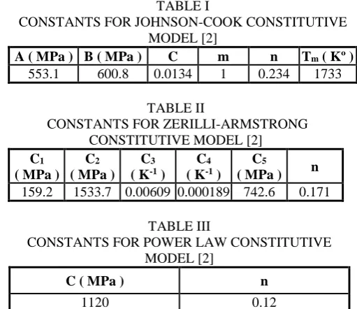
[image:2.595.298.554.294.515.2]The material coefficients used in calculating the Johnson-Cook, Zerilli-Armstrong and Power Law flow stress values are listed in Table 1 to 3.
TABLE I
CONSTANTS FOR JOHNSON-COOK CONSTITUTIVE MODEL [2]
A ( MPa ) B ( MPa ) C m n Tm ( Kº )
553.1 600.8 0.0134 1 0.234 1733
TABLE II
CONSTANTS FOR ZERILLI-ARMSTRONG CONSTITUTIVE MODEL [2]
C1
( MPa ) C2
( MPa ) C3
( K-1 )
C4
( K-1 )
C5
( MPa ) n
159.2 1533.7 0.00609 0.000189 742.6 0.171 TABLE III
CONSTANTS FOR POWER LAW CONSTITUTIVE MODEL [2]
C ( MPa ) n
1120 0.12
The next step was to compare the cutting forces resulting from the SPH method versus the FEM method versus empirical values. The same three different constitutive models were used for each simulation method.
The SPH method was also evaluated for its sensitivity to time scaling, and frictional behavior of tool-chip interface. Lastly, the effects of rake angle and tool tip radius on the stress distributions were investigated.
IV. RESULTS AND ANALYSIS
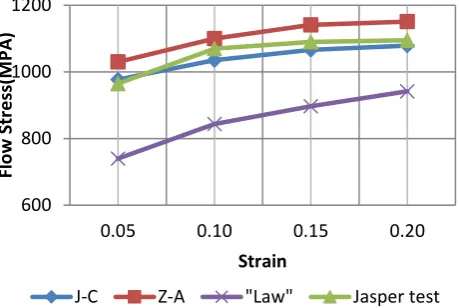
A. Flow Stress vs. Strain, Strain rate and Temperature during Cutting Process
Fig. 1. AISI 1045 Flow stress prediction by Z-A, J-C and Law models vs. Jasper empirical results at 20 ºC
[image:3.595.312.545.208.392.2]The same simulation was done at a room temperature of 400ºC. Thermal softening behavior of the material at higher temperatures was predicted well by the Z-A model. In contrast, the J-C model overestimated the flow stress by 200MPa at a room temperature of 400 ºC.
Fig. 2. AISI 1045 Flow stress prediction by Z-A and J-C models vs. Jasper empirical results at 400 ºC B. Force Analyses
In this section, the metal cutting forces predicted by the J-C, Z-A and Power Law constitutive material models using the SPH method were compared against both empirical values and results obtained by Kiliçaslan [1] using the Finite-Element Method with the same three models and conditions. Figure 3 and Table 4 compares the Tangential and Normal forces for each of the seven configurations.
TABLE IV
FORCE ANALYSIS OF EMPIRICAL VALUES VERSUS SPH AND FEM METHODS WITH VARIOUS
CONSTITUTIVE MODELS Machining Forces (Newtons)
Tangential Error Normal Error Ave. Error
Experimental 745 600
SPH (Z-A) 800 7% 504 -16% 12%
FEM (Z-A) 1224 64% 792 32% 48% SPH (J-C) 600 -19% 444 -26% 23%
FEM (J-C) 918 23% 570 -5% 14%
SPH (Law) 1192 60% 750 25% 43% FEM (Law) 852 14% 522 -13% 14%
The data shows that the using the SPH method with the Z-A model predicted the closest values to the experimental than the other models. The Z-A model overestimated the tangential forces by 7% and underestimated the normal force by 16%. The average error was 12% and was the lowest compared to any of the other models or methods. These errors may be partly attributed to the material model of the tool, which was assumed to be a rigid body. The friction model may have also affected the results, considering that it has a strong effect in the calculation of the cutting forces especially in case of normal forces.
Fig. 3. Force analysis of empirical values versus SPH, FEM and Power Law models
Moreover, some thermal and mechanical phenomena happening in the real metal cutting process such as tool wear, elastic recovery of workpiece, machined surface roughness and heat transmission between tool and workpiece and ambient, were not considered in this study. Despite these limitations, Z-A model is the best for analyzing the machining of AISI 1045 via SPH method. Therefore this model has been utilized for all the rest of the analyses.
C. Friction Analysis
The Ls-Dyna software allows friction to be defined specifically for static (FS) and dynamic friction (FD). The frictional model is restricted to a type of Coulomb friction, dependent on the relative velocity
|v
rel|
of the surface in contact. The overall friction coefficient follows the formula:µ
с= 𝐹
𝐷+ (𝐹
𝑆− 𝐹
𝐷)𝑒
−𝐷𝐶|𝑣𝑟𝑒𝑙|In this study, the simulations were performed with varying parameters for static and dynamic friction, as shown in Table 5. All the process parameters are identical except the friction coefficient.
TABLE V
COULOMB FRICTION PARAMETERS VALUES
Model type
𝑭
𝑺𝑭
𝑫1 0.5 0.8
2 0.5 0.3
3 0.6 0.5
4 0.4 0.5
5 0.5 0.5
600 800 1000 1200
0.05 0.10 0.15 0.20
Fl
o
w
Str
e
ss(M
PA
)
Strain
J-C Z-A "Law" Jasper test
600 800 1000 1200
0.05 0.10 0.15 0.20 0.25
Fl
o
w
Str
e
ss(M
PA
)
Strain
J-C Z-A Jasper test
745
600 800
504 1224
792
600
444 918
570 1192
750 852
522
0 200 400 600 800 1000 1200 1400
Tangential Normal
Exp. SPH (Z-A) FEM (Z-A) SPH (J-C)
[image:3.595.50.288.326.476.2]In the Figure 4 and Figure 5, the effects of each model number on the output forces can be seen. When FS is kept constant in cases 1, 2 and 5, there is no obvious trend with the output forces and are roughly constant. However, when FD is kept constant in cases 3, 4 and 5, the forces consistently increase with FS. Hence, the simulated cutting forces are more sensitive changes in the FS parameter versus FD parameter. This observation is consistent for both the tangential and the normal forces.
[image:4.595.307.551.84.220.2][image:4.595.45.292.167.296.2]
Fig. 4. Tangential force results of different model number
Fig. 5. Normal force results of different model number Thus, special care must be taken to calibrate the model for friction. It is noteworthy that the temperature during the cutting process predicted by the Finite Element Method is similar to prediction of the SPH method of around 555 ºC.
D. Mechanical Analysis – Rake Angle
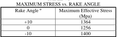
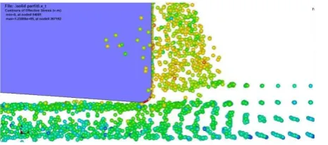
In this section, the influence of different rake angles on flow stress at the workpiece was investigated. Three types of rake angles were used: -10º, 0º, +10º. The effect of different rake angles on the cutting process is shown in Figure 6 to 8.
TABLE VI
MAXIMUM STRESS vs. RAKE ANGLE Rake Angle º Maximum Effective Stress
(Mpa)
+10 1364
0 1256
-10 1400
[image:4.595.46.290.266.431.2]It is apparent in Figures 6, for positive rake angles, that the stress field in the primary shear zone is narrower and the maximum stress is almost constant at 1360 MPa during the process. Also, it can be seen that its effects on the machined surface is more significant than at zero and negative rake angles. Most importantly, the propagation of the stress through the workpiece is lower than the other types in each step. This stress propagation may be useful to analyze the phenomena of strain hardening during machining.
Fig. 6. Effective Stress results of rake angle +10º
[image:4.595.302.552.282.413.2]Fig. 7. Effective Stress results of rake angle 0º
Fig. 8. Effective Stress results of rake angle -10º
It should be noticed that, the maximum value of the flow stress of the workpiece at zero rake angle of the tool is lower than the time that the rake angle is +10, but it is not constant like that and it is increasing gradually until the maximum value which is around 1250 MPa. Stresses has predicted, the FEM results is lower and is around 1220 MPa. The maximum value of the flow stress obtained at rake angle -10. It is much more than rake angle +10º and 0º because, the contact of the tool with the workpiece is in larger area at secondary shear zone when the rake angle is -10º. Although it is interesting that the highest stress in the primary shear zone has obtained at the positive rake angle. It
1 2
3
4 5
0 200 400 600 800 1000 1200
Ta
n
g
en
tia
l
Fo
rc
e
(
N ) 1
2
3
4
5
1 2
3
4 5
0 200 400 600 800
No
rm
a
l
Fo
rc
e
(
N ) 1
2
3
4
[image:4.595.309.549.472.592.2] [image:4.595.54.290.607.683.2]can be understood that the concentration of the stress occurred at the on the tool tip.
E. Mechanical Analysis – Tool Tip Radius
[image:5.595.48.291.194.300.2]In this section, the influence of the tool tip radius on the flow stress of the workpiece during metal cutting process has been investigated. For this purpose, three different tool tip radius were used, specifically 5 µm, 50 µm and 68µm. All of the other parameters are identical with the settings of the empirical works cited in the previous sections.
[image:5.595.39.297.394.469.2]Fig. 9. Effective Stress results of tool tip radius of 5µm Tool tip radius has an important effect on the workpiece stress during the cutting process. As can be seen in Table 7, the stresses during machining increase as the tool tip radius is increased.
TABLE VII
MAXIMUM STRESS vs. TOOL TIP RADIUS Tool Tip Radius (µm) Maximum Effective Stress
(Mpa)
5 1182
50 1189
68 1232
For a tool tip radius of 68µm, the particle fringe component shows the stresses on the flank surface of the tool and on secondary shear zone is lesser than the time that the tool tip radius is 5µm. But it can be observed that the concentration of the stresses on tool tip is higher than the time the tool tip radius is 5µm. Stresses has predicted the FEM results is lower and is around 1220 MPa.
Fig 10. Effective Stress results of tool tip radius of 68µm It can be seen that by increasing the tool tip radius, plastic deformation on the machined surface and in the secondary shear zone has increased as well. This is due to the stress concentration getting much higher on the tool tip when increasing the tool tip radius, which causes small cracks and distortion on tool edges.
V. CONCLUSION
It has been found that the SPH method used with the Z-A model is able to give the most accurate results in simulating the machining of AISI 1045. The study also corroborates the finding of Jasper that the prediction using the Z-A model for flow stress versus temperature is more accurate than the J-C model for AISI 1045 material. In the case of friction analysis, it can be observed that the effect of static coefficient is much more than dynamic coefficient. It can be seen that higher values of friction coefficients cause an irregular shape and size on chip formation so the coefficient obtained from analytical formulations may not be used in simulation analysis.
In the section analyzing the effects of mechanical parameters, it has been concluded that the rake angle has a big influence on the flow stress of the material in metal cutting process. It was shown that the maximum stress in the primary shear zone and the tool tip occurred when the rake angle is positive. Also, the maximum values of flow stress at the secondary shear zone were obtained when the rake angle of tool is negative, where the contact surface between tools and workpiece were highest. By increasing the tool tip radius the stress concentration is increased at the tool tip, causing small cracks and distortion on tool edges.
VI. RECOMMENDATION
For future researches the study on oblique cutting process and further study on thrust forces in 3D simulation analysis is recommended. Also segmented chip formation by work on machining of hard materials such as Titanium alloys and frictional behaviour can be studied by researchers. Another shortcoming that can be studied more in the future is the temperature distribution in SPH method which is not applicable yet by this version of Ls-Dyna software. SPH method can be applied also for the other machining processes such as milling and drilling. Experimental measuring of chip geometry and cutting forces must also be performed in order to get a realistic comparison between analyses and experiments.
NOMENCLATURE
𝛼 Relief angle, ( º )
𝛾 Rake angle, ( º )
𝑟 Tool tip radius, ( mm ) 𝜌 Density, ( Kg / M3 )
𝐸 Elastic modulus, (Gpa)
𝑎𝑣 Thermal Expansion, ( 1/ º C)
𝑘 Thermal Conductivity, ( N / Sec / º C ) 𝐶𝑝 Heat Capacity, ( N/mm2 º C )
𝑣 Poisson's ratio
𝐺 Shear Modulus, 𝐺 ( GPa ) 𝑇𝑚 (º C ) Melting Point, (º C ) 𝑉 ( m/min ) Cutting Velocity, ( m/min )
𝑡1 Depth of Cut, ( mm )
𝑑𝑤 Width of Cut, ( mm )
𝑇 Temperature, (º C)
𝐹𝑇 Tangential Force, ( N )
𝐹𝑁 Normal Force, ( N )
[image:5.595.67.300.571.674.2]REFERENCES
[1] Cenk K., (2009). Modeling And Simulation Of Metal Cutting Finite Element Method. A thesis submitted to the graduate school of engineering and sciences of izmir institute of technology in partial fulfillment of the requirements for the degree of Master of science. [2] Jaspers, S.P.F.C. and Dautzenberg, J.H. (2002).
Material Behaviour in Conditions Similar to Metal Cutting; Flow Stress in the Shear Zone.Journal of Materials andProcessing Technology 122: 322-330.
[3] Filice, L., Micari, F., Rizutti, S. and Umbrello, D. (2007). A Critical Analysis On the Friction Modelling in Orthogonal Machining. International Journal ofMachine Tools and Manufacturing 47: 709-714.
[4] Limido J, Espinosa C, Salaun M (2007) SPH method applied to high speed cutting modeling. Int. J. Mech. Sci., Volume (49), 898-908.
[5] Morten F. Villumsen, Torben G. Fauerholdt, LS-DYNA Anwenderforum, Bamberg (2008).
[6] Bagci E. (2010). 3-D numerical analysis of orthogonal cutting process via mesh-free method.International Journal of the Physical Sciences Volume 6 (6), pp. 1267-1282.
[7] Lacome JL (2001a). Smooth Particle Hydrodynamics-Part II.FEA Newsletters.6-11.
[8] Lacome JL (2001b). Smooth Particle Hydrodynamics-Part II.FEA Newsletters.6-11.
[9] Lacome JL (2002). Smoothed particle hydrodynamics (SPH): A New Feature in LS-DYNA. 7th International LS-DYNA Users Conf. Dearborn, Michigan, Volume(7), 29–34.
[10] Oxley, P.L.B. (1990), Mechanics of Machining: An Analytical Approach to Assessing Machinability. Journal of Applied Mechanics, Volume (57), 253.
[11] Hallquist JO (1998). LS-DYNA Theoretical Manual. LSTC, Livermore, CA, USA.