Active speaker localisation and tracking using audio and video

(1)

and Tracking using Audio and

Video

A dissertation submitted to the University of Dublin for the degree of Doctor of Philosophy

Damien Kelly

Trinity College Dublin, March 2010

(2)

(3)

This thesis is concerned with the problem of tracking active speakers using audio and video data. Particular focus is placed on the task of tracking the current active speaker in a lecture room environment using multiple cameras and multiple microphones. A database of lecture recordings corresponding to this scenario from the European Integrated Project, Computers in the Human Interaction Loop (CHIL) is used to support work presented throughout the thesis.

Within the lecture room environment, the problem of extracting reliable audio and video based features for detecting people is explored. In the audio domain, the use of time-delay estimates from multiple pairs of microphones is examined for localising active speakers. Fun-damental limitations on localisation accuracy using this approach are also discussed. In the video domain, background modelling, face detection and skin colour detection are considered as candidate features for the visual detection of people. A new skin colour model is introduced which models for the non-linear dependence of skin-tone on luminance and is shown be eﬀective in modelling skin colour under low illumination. Following the evaluation of audio and video features for locating people, a review of existing techniques which aim to fuse audio and video information for tracking is presented.

This thesis makes two critical analyses in relation to the joint audio-video based localisation problem. The first analysis examines the expected accuracy of audio-based localisation using multiple microphones and video-based localisation using multiple cameras. Within this analy-sis, the theory of estimating localisation uncertainty for both localisation techniques is unified under a common framework. Using this, single modality localisation is compared to localisation through different audio-video based fusion strategies. The different fusion strategies evaluated are the fusion of audio and video location estimates in the positional domain, the audio domain and the video domain. For each of these fusion methods, it is found that little is to be gained in terms of localisation accuracy through a fusion based approach, in comparison to the accuracy of single modality video-based localisation.

(4)

scenarios which consider minimising localisation uncertainty over user deﬁned presenter and audience areas.

(5)

I hereby declare that this thesis has not been submitted as an exercise for a degree at this or any other University and that it is entirely my own work.

I agree that the Library may lend or copy this thesis upon request.

Signed,

Damien Kelly

(6)

Firstly, I would like to express sincere gratitude to my supervisor Prof. Frank Boland for his help, encouragement, patience and guidance throughout the course of my PhD. His encourage-ment, in particular, led me towards the path of postgraduate research and for this I am truly grateful. An enormous amount of thanks is also due to Prof. Anil Kokaram, for many inspiring discussions, ideas and invaluable advice. Dr. Fran¸cois Piti´e and Dr. Dave Corrigan were also extremely generous with their time and help over the last number of years and I thank them hugely for that.

Thanks must also go to both the staﬀ and post-graduate students of the Electronic & Elec-trical Engineering Department in Trinity College for their help and also for creating such a friendly and lively working atmosphere. I would like to thank, Bernadette, Conor, Robbie and Nora for their help throughout the years.

A special thanks goes to the members of the SIGMEDIA group and other members of the lab, especially; Dr. Naomi Harte, Gavin, Dan, Deirdre, John, Darren, Gary, Ricardo, Cedric, Craig, Claire, the two Andrews, Liam, Kangyu, Mohamed and Steven. To past members of the lab; Angela, Denis, Deepti and Daire, I thank you also. It has been a privilege to work in the company of such helpful, friendly and engaging people.

As a postgraduate research student I have beneﬁted from the support of the Irish Research Council for Science, Engineering and Technology (IRCSET) and also Science Foundation Ireland (SFI). Many thanks to these organisations for their support.

(7)

Contents vii

List of Acronyms xi

List of Figures xiii

List of Tables xvii

1 Introduction 1

1.1 CHIL Database . . . 3

1.2 Thesis Outline . . . 4

1.3 Contributions . . . 7

1.3.1 Publications. . . 7

2 Audio and Video Features for Active Speaker Localisation 9 2.1 Audio Features . . . 10

2.1.1 Propagation of Sound in Rooms . . . 11

2.1.2 Microphone Array Signal Processing . . . 15

2.1.3 Time-delay based Localisation . . . 17

2.1.4 Localisation through Sound Intensity Diﬀerences . . . 24

2.1.5 Steered Response Power based Localisation . . . 25

2.2 Video Features . . . 27

2.2.1 Background Modelling . . . 29

2.2.2 Face Detection . . . 32

2.2.3 Skin Colour Modelling . . . 36

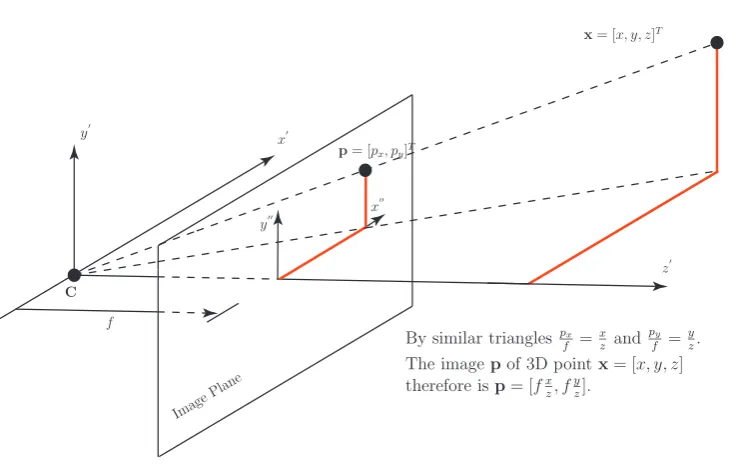
2.2.4 Camera Measurement Function . . . 42

2.3 Final Comments . . . 48

3 Joint Audio-visual Active Speaker Tracking 51 3.1 Bayesian State Sequence Estimation . . . 53

3.1.1 Recursive Bayesian Filter . . . 54

3.1.2 The Kalman Filter (KF). . . 55

(8)

3.1.3 Kalman Filters for Audio-based Tracking . . . 60

3.1.4 The Particle Filter . . . 61

3.1.5 Grid-based Approximation . . . 63

3.2 Combining Audio and Video Observations for Tracking. . . 64

3.2.1 Simple Average . . . 64

3.2.2 Audio-video Fusion using Kalman Filters . . . 65

3.2.3 Audio-video Fusion using Particle Filters . . . 68

4 Analysis of Audio-Visual Source Localisation Accuracy 77 4.1 Uncertainty Mapping. . . 79

4.1.1 Linear Approximation Mapping. . . 80

4.2 Audio-based Measurement Function . . . 81

4.3 Video-based Measurement Function . . . 83

4.4 Conﬁguration of Experimental Audio-Video Localisation System . . . 84

4.4.1 Validity of First Order Error Propagation . . . 86

4.4.2 Comparison with the Unscented Transform . . . 87

4.5 Comparative Error Analysis and Discussion . . . 93

5 Optimal Microphone Placement 101 5.1 Localisation Accuracy of a Microphone Array Conﬁguration . . . 105

5.1.1 Univariate Measures of Localisation Uncertainty . . . 105

5.1.2 The Objective Function . . . 106

5.2 Modelling Uncertainty on the Time-delay Estimates . . . 109

5.2.1 The Correlator Performance Estimate (CPE) . . . 109

5.2.2 Speaker and Microphone Directivity Characteristics . . . 112

5.3 A Simulated Annealing based Approach . . . 113

5.3.1 Basic Simulated Annealing Algorithm . . . 114

5.3.2 Proposed Simulated Annealing Algorithm . . . 115

5.4 Results. . . 116

6 Voxel-based Viterbi Active Speaker Tracking V-VAST 123 6.1 Probabilistic Framework . . . 125

6.1.1 Audio-based and Video-based Likelihood Functions. . . 127

6.1.2 Priors . . . 131

6.2 Determining Candidate Speaker Positions . . . 134

6.2.1 Extracting Connected Skin Regions . . . 134

(9)

6.2.3 Extracting Connected Voxel Regions . . . 135

6.2.4 Ellipsoid Fitting . . . 136

6.3 Joint Maximum a posteriori (MAP) Estimation using the Viterbi Algorithm . . 139

6.4 Visually Segmenting the Active Speaker . . . 141

6.4.1 Determining theBest Camera View . . . 141

6.5 Evaluation of Tracking Accuracy . . . 142

6.6 Visual Segmentation Results. . . 146

6.6.1 Single Speaker Case . . . 147

6.6.2 Speaker Switching Case . . . 151

7 Discussion & Conclusion 161 7.1 Future Work . . . 163

A Approximation of the First Order Derivative of the Inverse Time-Delay Mea-surement Function 167 B Audio-Video Localisation: Experimental Setup 169 B.1 Video Cameras and Microphones . . . 169

B.2 Note on the Optimality of the Experimental Setup . . . 169

C Complete Set of Seminar Tracking Results 173

D Multi-camera Calibration Procedure 181

(10)

(11)

CC Cross-Correlation

GCC Generalised Cross Correlation

PHAT Phase Transform

DOA Direction Of Arrival

𝑅𝑇60 Reverberation Time

SRP Steered Response Power

TDE Time Delay Estimate

SA Simulated Annealing

ML Maximum Likelihood

MAP Maximum a posteriori

SNR Signal to Noise Ratio

CHIL Computers in the Human Interaction Loop

ELRA European Language Resource Association

KF Kalman Filter

PF Particle Filter

EKF Extended Kalman Filter

IEKF Iterated Extended Kalman Filter

UKF Unscented Kalman Filter

MSE Mean Square Error

UT Unscented Transform

(12)

MAE Mean Absolute Error

CRLB Cram´er-Rao Lower Bound

CPE Correlator Performance Estimate

SRR Signal-to-Reverberant Ratio

GCC-PHAT Generalized Cross-Correlation with Phase Transform

SRP-PHAT Steer Response Power - Phase Transform

SA Simulated Annealing

CP Constant Position

CV Constant Velocity

CA Constant Acceleration

HCI Human Computer Interaction

SIS Sequential Importance Sampling

STFT Short Time Fourier Transform

LTI Linear Time Invariant

PCA Principal Component Analysis

V-VAST Voxel-based Viterbi Active Speaker Tracking

GCF Global Coherence Field

(13)

1.1 Sample frames and room layout of the CHIL room. . . 5

2.1 Illustration of the relative time delay and Direction Of Arrival (DOA) at a pair of microphones. . . 19

2.2 Time-delay and DOA localisation techniques. . . 20

2.3 Localisation using interaural level diﬀerences. . . 25

2.4 Example of diﬃcult face detection problems in the lecture recordings of the CHIL database. . . 29

2.5 Example of the performance of various background estimation techniques. . . 32

2.6 Sample of skin colour pixels in 𝑅𝐺𝐵 space captured under varying illumination. 38 2.7 Non-linear dependence of skin tone on illumination in diﬀerent colour spaces . . 39

2.8 Estimating the correlation between the 𝑅, 𝐺 and 𝐵 components of skin colour by two polynomials. . . 40

2.9 Sample frame from the CHIL database together with a scatter plot of the frame’s pixels in the RGB colour space . . . 43

2.10 Comparison of the proposed skin colour detection technique to that of Hsu et al. [156] and Jones et al. [120] . . . 44

2.11 Pinhole camera model. . . 45

2.12 Camera ray as a parameterised line in 3𝐷 space. . . 46

3.1 Simulated evaluation of Divergence in the Kalman Filter (KF). . . 59

3.2 Centralised and Decentralised Joint Kalman Filters (KFs).. . . 66

3.3 Illustrated example of diﬀerent body shape models for particle ﬁlters. . . 72

4.1 Mapping uncertainty between audio, video and positional domains. . . 82

4.2 Experimental setup used in the evaluation of audio-visual source localisation. . . 85

4.3 Point correspondences used in calibrating the cameras in the evaluation of audio-visual source localisation. . . 87

4.4 Evaluation of ﬁrst order error propagation in an audio-video based localisation system. . . 91

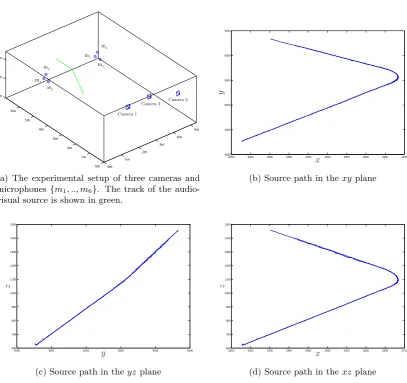
4.5 Audio-video source localisation of a moving audio-visual source. . . 94

(14)

4.6 Comparison of audio-visual source localisation and various fusion based

localisa-tion strategies. . . 95

4.7 Comparison of audio-based, video-based and fusion-based localisation performance. 96

4.8 The results of audio-based, video-based and fusion-based localisation in the𝑥,𝑦

and 𝑧 dimensions . . . 100

5.1 Parameterised inverted T-shaped microphone array. . . 103

5.2 Examination of ∑_𝑖𝑡𝑟(Σx𝑖)2 as a cost function in the microphone array conﬁgu-ration optimisation problem. . . 108

5.3 Three regions of operation for an unbiased time-delay estimator as deﬁned by the

Correlator Performance Estimate (CPE). . . 110

5.4 The Cram´er-Rao Lower Bound (CRLB) and Correlator Performance Estimate

(CPE) for time-delay estimation using cross-correlation in a reverberant environ-ment . . . 112

5.5 Optimising the conﬁguration of 4 inverted T-shaped microphone arrays over

sym-metric audience and presenter regions. . . 118

5.6 Optimising the conﬁguration of 4 inverted T-shaped microphone arrays over

non-symmetric audience and presenter regions. . . 120

5.7 Optimising the conﬁguration of 4 inverted T-shaped microphone arrays within

user speciﬁed regions for audience and presenter localisation . . . 121

6.1 Block diagram of the Voxel-based Viterbi Active Speaker Tracking (V-VAST) algorithm and sample output composite view video sequence. . . 126

6.2 Example form of the audio-based likelihood function used in V-VAST . . . 129

6.3 Example form of the motion prior used by V-VAST. . . 132

6.4 Illustrative example of ﬁtting an ellipsoial head model to the detected 3𝐷 fore-ground. . . 137

6.5 Head detection example using detected skin colour regions in four views and an

ellipsoidal head model. . . 138

6.6 Illustration of the joint trellis structure of the Viterbi tracking problem in V-VAST.140

6.7 Criteria for choosing the best view of the active speaker. . . 143

6.8 Visually segmenting the active speaker in theseminar 2004-11-12 A segment2

sequence of the CHIL database. . . 149

6.9 Visually segmenting the active speaker in theseminar 2004-11-12 B segment1

sequence. . . 150

6.10 Visually segmenting the active speaker in theseminar 2004-11-11 C segment1

6.11 Occlusion problem in theseminar 2004-11-11 C segment1 sequence. . . 153

6.12 Visually segmenting the active speaker in theseminar 2004-11-11 A segment4

(15)

6.13 Visually segmenting the active speaker in theseminar 2004-11-12 B segment3

6.14 Visually segmenting the active speaker in theseminar 2004-11-12 B segment2 sequence of the CHIL database. . . 157

6.15 Skin colour distortion problem in the seminar 2004-11-12 B segment2 se-quence. . . 158

B.1 Illustration of the unoptimised and optimised microphone array positions for the experimental setup used in chapter 5. . . 172

C.1 Tracking results forseminar 2004-11-11 A segment1. . . 175

C.3 Tracking results forseminar 2004-11-11 B segment1 . . . 176

C.5 Tracking results forseminar 2004-11-11 C segment1 . . . 177

C.6 Tracking results forseminar 2004-11-11 C segment2 . . . 177

(16)

(17)

3.1 Transition matrices for a constant position model CP, constant velocity model

CV and constant acceleration model CA. . . 58

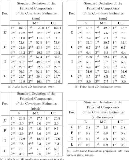
4.1 Examining covariance values in the evaluation of ﬁrst order error propagation in

an audio-video based localisation system. . . 92

6.1 Speaker activity states deﬁned over three time steps. . . 127

6.2 Results corresponding to the visual person tracking task of the CHIL 2005

eval-uation. . . 146

6.3 Results corresponding to the visual person tracking task of the CHIL 2005

eval-uation using the 3𝐷global mean error.. . . 147

B.1 Description and positions of the six microphones and three video cameras used

in the analysis of audio-visual source localisation. . . 170

B.2 Positions of both the calibration training points and test points used in calibrating the video cameras . . . 171

(18)

(19)

1

Introduction

Continuing advancements in technologies for transmitting multimedia over the Internet, opens a gateway for universities to expand their campus beyond its physical limits and to start offering educational content online. Recently, universities have begun to try and avail themselves of this new opportunity, which is changing the landscape of traditional education. New methods of teaching through this medium are evolving to meet the growing demands of students who desire greater flexibility in education. This has seen the emergence of web-based course content focused towards supplementing normal face-to-face lectures or facilitating distance education and on-demand learning. This represents a new avenue in education popularly known as eLearning. Within eLearning, two predominant categories exist: synchronous and asynchronous. Syn-chronous eLearning refers to the live presentation of educational content such as the streaming of multimedia to a remote user. The aim is to provide the user with an equivalent learning experience to that of the in-class participant such as, for instance, the opportunity to interact and ask questions. For many universities the ultimate goal in their eLearning ambitions is to enable students to attend lectures remotely using the Internet in a synchronous manner. How-ever, few have the infrastructure to support this and network technologies have still not reached sufficient bandwidth capabilities to communicate all the necessary audio, video and additional multimedia.

In contrast to synchronous eLearning, asynchronous eLearning is concerned with the pre-sentation of educational resources in an oﬄine manner where the material is not viewed live, but on-demand. Recording lectures and providing them online for asynchronous viewing is a more realistic option for universities at present in comparison to the synchronous alternative,

(20)

since it is possible now through existing technology. Presently, many universities oﬀer recorded lectures online through partnerships with Apple iTunes U [11] or Google’s youtube EDU [67]. In addition to this, some universities even maintain their own video-on-demand servers supply-ing recorded lectures such as, Princeton University’s WebMedia [149], University Cambridge’s CamTv [28], Massachusetts Institute of Technology’s OpenCourseWare [127] and University California Berkley’s WebCast [185]. As an asset to students for learning, the ability to access recordings of lectures is highly valued since it augments the learning experience and can im-prove student performance [81,158]. It is not surprising therefore, that the demand for such asynchronous online lecture content is ever increasing [142].

Recording lectures and making them available online requires a significant amount of ef-fort and commitment on a university’s behalf. Commercially available systems exist such as, Panopto’s CourseCast [145], Sonic Foundary’s MediaSuite [173], Echo360’s EchoSystem [49] and Tegrity Campus [181] which enable lectures to be captured automatically without the need for any technical expertise. Some universities have even developed their own systems for lecture capture such as the eClass system used by Georgia Institute of Technology [81]. In general, these systems require the presenter to remain within the field of view of a fixed camera re-stricting their movements to a small area. Student opinions have shown that rere-stricting the presenter’s movements can significantly reduce the perceived classroom experience [130]. One commercially available system which places less constraints on a presenter’s movements is Au-toauditorium [112]. This is a purely vision based system for tracking the presenter over a large area. The system however is specifically designed for tracking the presenter and does not suf-ficiently address the task of tracking audience interactions. This is a current limitation since interaction from an audience is a significant element of many lecture presentations. The ulti-mate goal in the production of video lectures for viewing offline, is to convey exactly that of the in-classroom experience. In-class participants have the freedom to visually follow conversational interactions. If this aspect of a lecture is not conveyed in a recording, the offline viewer’s learn-ing experience is reduced in comparison to that of the in-class participant. Furthermore, it is the opinion of professional video producers that lecture recordings which visually capture both the audience and the presenter offer a more enjoyable viewing experience than recordings which simply capture the actions of the presenter [150].

(21)

What is needed therefore, is an intelligent unobtrusive system for automatically capturing all aspects of a lecture. By unobtrusive it is meant that the system does not inﬂuence how the lecture should be conducted in order for the capture to be successful. The lecture should be able to proceed under normal circumstances and not be aﬀected in any way by the capturing system. Clearly an important component of such a system is the ability to track the position of the current active speaker. This is important because it is normally the case that the focus of communication in a lecture is at the position of the current active speaker.

In recent times, more intelligent automated lecture capturing systems have begun to emerge for automatically capturing lectures such as Microsoft’s lecture capture system [27]. This system represents one of the most sophisticated automated lecture capturing systems in use. This particular tracking algorithm relies on data from two cameras and a microphone array. One camera is focused on the presenter and the visual data from this camera is used specifically for the tasks of tracking the presenter and appropriately capturing the presenter’s actions. The second camera which the system employs is assigned to the task of visually capturing the audience members. Individual audience members are located when they ask questions by using the audio data captured at the microphone array. Only the audio data is used to locate audience members who are speaking and this information is used to direct the audience camera to the person who is speaking. As will be highlighted in this thesis, accurate and reliable audio-based localisation can be notoriously difficult to achieve in lecture room environments. A system which relies on audio data only to locate speakers is likely to be unreliable. The designers of the Microsoft lecture capturing system acknowledge this and highlight this point as a significant limiting factor in their system’s ability to accurately and consistently capture questions from audience members [27].

Recently however, researchers have begun to examine combining audio and video based measurements for tracking. The basic idea in this approach is that both audio and video can be used to complement each other when applied to tracking and improved reliability and accuracy can be achieved. This thesis is concerned with the combined use of audio and video for tracking. More speciﬁcally, this thesis is concerned with using both audio and video for tracking the current active speaker in a lecture room environment. The motivation for this work is the development of automated systems for capturing lectures and creating lecture recordings suitable for presentation over the Internet in eLearning applications for the purpose of archiving.

1.1

CHIL

Database

(22)

the European Commission’s Sixth Framework Programme. It began in 2004 with the objective to “create environments in which computers serve humans who focus on interacting with other humans as opposed to having to attend to and being preoccupied with the machines themselves”. The main focus in this project was towards the office and lecture room scenario. Over the course of the project until it ended in 2007 several evaluations were conducted to examine various technologies in a broad range of tasks including audio-based and video-based tracking; joint audio-video based tracking; speech and person recognition; gesture recognition; automated transcription; activity detection and audio-visual Scene Analysis. These evaluations began with the first evaluation campaign in 2004 and each year after until 2007. For each evaluation a specific evaluation package of annotated audio and video recordings complete with specific metrics and ground truth for each concerned task were created. These packages have recently become available through the European Language Resources Association [50].

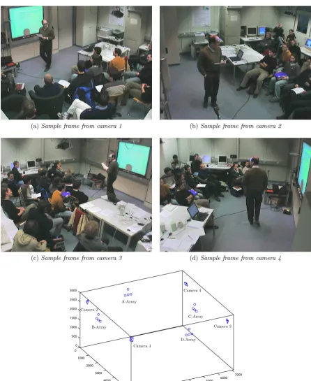
Relevant to the lecture scenario of interest to this work is the 2005 evaluation package. Within this package is a set of multi-channel audio and multi-camera video recordings of five seminars made at ISL, Universität Karlsruhe in November 2004. The multi-channel audio data consists of various different 44.1𝑘𝐻𝑧 recordings including a 64-channel microphone array; 4 T-shaped microphone arrays of 4 microphones each; 5 single table-top microphones and a close-talking microphone. The video data consists of 15𝑓 𝑝𝑠recordings from 4 cameras positioned in each of the four corners of the seminar room. A sample of the four camera views of a seminar recording and an illustration of the sensor layout within theCHIL lecture room is shown in figure1.1.

1.2

Thesis Outline

The following outlines the structure of the thesis,

Chapter 2: Joint Audio-visual Active Speaker Tracking

A review of audio and visual features useful for tracking active speakers is presented in chapter

2. In the audio domain, features arising from the capture of a speech source signal by multiple microphones are described. It is examined how these can be used in localising a speech source. The challenges faced in a lecture room environment such as room reverberations and fundamental limitations in achieving accurate and reliable localisation are discussed.

(23)

(a)Sample frame from camera 1 (b)Sample frame from camera 2

(c)Sample frame from camera 3 (d)Sample frame from camera 4

0 1000

2000 3000

4000 5000

0 1000

2000 3000

4000 5000

6000 7000 0

500 1000 1500 2000 2500 3000

B-Array

A-Array

C-Array

D-Array Camera�2

Camera�4

Camera�3

Camera�4

[image:23.595.89.536.109.655.2]

(e) The setup of the four cameras and four T-shaped micro-phone arrays of theCHILroom.

(24)

Chapter 3: Audio and Video Features for Active Speaker Localisation

In this chapter, a Bayesian framework for active speaker tracking using audio data is established. Audio-based tracking ﬁlters are reviewed in reference to the presented probabilistic framework. Consideration is given to persistent problems in tracking such as motion modelling and the chal-lenge in choosing suitable models for motion. It is shown how the presented tracking framework can be easily extended to include video information. Existing joint audio-video based active speaker tracking techniques are explored within this framework and common strategies for the fusion of audio and video information are described.

Chapter 4: Analysis of Audio-Visual Source Localisation Accuracy

This chapter compares the performance of audio-based localisation using multiple microphones and video-based localisation using multiple cameras in a typical lecture room. Also examined is the accuracy of localisation through the fusion of the estimates from both modalities. In the evaluation, the task examined is that of localising an audio-visual source along a 3D track.

Within this chapter, the theory of uncertainty propagation for estimating the localisation accuracy through multiple cameras and multiple microphones is uniﬁed under a common frame-work. It is through the use of this theory that the comparative analysis of localisation accuracy is made. It is shown that audio contributes little in terms of accuracy when fused with video for localisation.

Chapter 5: Optimal Microphone Placement

This chapter explores the effect of microphone array positions on the expected accuracy of audio-based localisation. A simulated annealing based algorithm is introduced for automat-ically optimising the positions of the microphone arrays. The analysis is presented from a theoretical viewpoint. The work draws on existing mathematical theory defining lower bounds on localisation accuracy in a reverberant environment. These bounds are further developed to include important aspects which influence localisation performance such as the relative angles between the speakers and the microphones. The CHIL lecture room is examined for a hypo-thetical lecture scenario and the expected localisation accuracy for the given microphone array setup is examined. Using this example, the usefulness of the proposed algorithm for optimising the microphone array positions is shown.

Chapter 6: Voxel-based Viterbi Active Speaker Tracking V-VAST

(25)

of a user deﬁned main view and an automatically segmented view of the current active speaker.

V-VAST operates oﬀ-line as a post production step applied to multi-view lecture recordings. In visually segmenting the active speaker from the multiple views available, V-VAST aims to extract thebest view of the active speaker which is deﬁned as the view in which their face is most visible. The algorithm is extensively tested on multi-view lecture recordings from theCHIL2005 evaluation database demonstrating consistently accurate and reliable tracking performance.

Chapter 7: Discussion & Conclusion

The ﬁnal chapter of the thesis provides a summary of the main results and discusses their relevance and signiﬁcance. Future work and future directions for audio-visual active speaker tracking are also suggested to the reader.

1.3

Contributions

The contributions oﬀered by the work in this thesis are summarised in the following.

• A new skin colour model is presented which models for the non-linear dependence of skin-tone on luminance.

• The analysis of localisation uncertainty in multi-camera and multi-microphone systems is uniﬁed under a single framework

• A simulated annealing algorithm is introduced for determining the optimal positions of multiple microphone arrays for minimising localisation uncertainty.

• A new audio-video based active speaker tracking algorithm calledV-VASTis proposed for generating a composite view video sequence from a multi-view lecture recording.

1.3.1 Publications

Some of the above works and others arising from this thesis have appeared in the following publications.

[39] D. Kelly, F. Boland. Motion Model Selection in Tracking Humans. Irish Signals and Systems Confonerence (ISSC), pages 363-368, 2006.

(26)

(27)

2

Audio and Video Features for Active Speaker

Localisation

In this chapter, a review is presented of different audio and video based features which can be used for localising active speakers. The first section of this chapter examines audio-based features. In the audio domain, the specific use of multiple microphones for localising active speakers is examined. Numerous features arise from the capture of a speech source by multiple spatially separated microphones, which can be used to locate the source. An overview of these features is presented and how they can be used in localising active speakers is described. Also discussed, are aspects of the lecture room environment such as its acoustic properties which fundamentally limit the accuracy and usefulness of these localisation methods.

The second section of this chapter is dedicated to the analysis of visual features for detecting people using cameras. The multi-camera localisation problem is considered. In addition to the diﬃculties presented by the multi-camera scenario, the challenges of detecting people reliably in lecture rooms are explored. A new skin colour model is introduced for use in detecting face regions within a scene which is employed later in theV-VAST tracking algorithm introduced in chapter 6.

This chapter also acts as background to chapter3 which analyses the combination of audio and video features for tracking. It is not the aim of presented material in this chapter to be exhaustive. Instead, it focuses on introducing the localisation problem, basic terminology and feature extraction techniques which will be referred to in later chapters.

(28)

2.1

Audio Features

Humans like many animals in nature posses the innate ability to locate sound sources in three-dimensional space. This is achieved through binaural hearing whereby spatial information is extracted from the sound source received at the two ears. This task is performed with relative ease, often in very noisy environments and even in the absence of sight. In many applications; particularly those which aim to interact with or serve people, the ultimate goal is to fully replicate the binaural hearing ability observed in nature. Research eﬀorts over several decades have been dedicated to examining how such spatial information can be extracted from audio signals using multiple microphones.

Up until now this has not been achieved, as many aspects of how humans achieve binaural localisation remain unknown. What is presently known however, is that in locating acoustic sources, humans rely on at least two spatial cues. These cues arise due to the spatial separation of the ears causing sounds to be received at the ears, at different points in time. This results in a relative time delay between the two received sounds known as the interaural time difference. The second cue which humans use which is also due to the spatial separation of the ears, is the relative difference in the intensity of the sound received by each ear. This cue is known as the interaural intensity difference or interaural level difference.

Using two spatially separated microphones, one can aim to localise an acoustic source by extracting similar spatial cues from a source signal received by the microphones. The micro-phones can be used to indicate the sound intensity observed at their positions in a room. Both this cue and the relative time delay between the received signals can be used to indicate the direction of the source to the microphones. Indeed, this analysis is not restricted to just two mi-crophones but multiple pairs of mimi-crophones and arrays of mimi-crophones can be used in achieving the localisation task.

In the following sections, the use of multiple microphones for audio-based localisation is described. It is examined how the time-delays between multiple microphones and the diﬀerences in sound intensity observed by multiple microphones can be used to localise acoustic sources. The presentation will focus in parts on the general problem of localising acoustic sources. Of course, in this thesis the acoustic source will correspond to an active speaker. Where describing an active speaker simply as an acoustic source is too general, speciﬁc problems relating to active speaker localisation will be addressed.

Room Acoustics

(29)

as loudness is related to the sound power 𝑃 produced by the source. A 10𝑊 sound source for instance, will produce a sound which will be perceived as louder than a 1𝑊 sound source.

Sound Intensity

The perceived loudness of a sound is not only dependent on𝑃 but also the distance to the source. A sound source that is heard close to its source appears louder to a listener than the same sound heard from far away. The measurable quantity which relates loudness to the distance from the source is the sound intensity. The intensity of a sound at a particular point within a room is determined by the sound power 𝑃 and also by eﬀective area over which 𝑃 is dispensed. If an omni-directional source is assumed; that is, one which propagates sound waves equally in every direction, then𝑃 is dispersed over a spherical region. The area of this spherical region is equal to 4𝜋𝑟2 where 𝑟 is the distance of the sound source to the point where the sound intensity is to be measured. It is important to note that sound intensity is a vector quantity. It is common for sound intensity to be measured perpendicular to the eﬀective spherical area of 𝑃. This convention is also maintained in this thesis when referring to sound intensity and is denoted as the one-sided (one-direction) sound intensity. By this, the sound intensity 𝐼_𝑑 at a distance 𝑟

from a source is deﬁned as [73, Chapter 5], [4, Chapter 6],

𝐼𝑑=

𝑃

4𝜋𝑟2 (2.1)

This states that the observed sound intensity is inversely related to the distance to the source (𝑟) squared. This is known as the inverse square law of sound propagation.

2.1.1 Propagation of Sound in Rooms

Once a sound is introduced into a room it propagates as a wave, which in a normal room will travel at a speed of 343𝑚𝑠−1. As a wave, it is subject to all forms of wave distorting phenomena such as refraction, diffraction, interference and reflection. The actual room environment; its contents and structure, will dictate whether all or only some of these distortions are observed. Such factors will also dictate the extent of these distortions. In the lecture room environment concerned in this thesis, the presence of people, desks, chairs and structures such as walls mean that all the mentioned wave distortions are likely to be observed. As a result, the sound observed by a microphone at any point in the room will be different to that of the emitted sound.

Reverberation

(30)

or poorly surfaces within a room can absorb sound energy. Highly reflective surfaces within a room lead to a highly reverberant environment. The consequence of multiple reflected sound waves corresponding to the source is that it is difficult to discern the true sound wave from that of its reflections. Effectively, reverberation results in multiple “virtual” source locations from which the true source localisation must be determined.

A Model of Sound Propagation

It is common practice to apply a systems based approach to model the distorting eﬀects of a room on an emitted sound wave. In this approach, the room is modelled as a system with an input corresponding to the sound source and an output corresponding to the distorted sound wave. In relation to the acquisition of a sound wave by a microphone, we will consider the output of the system model as that observed by a microphone placed within the room.

A complete system model should reflect all of the relevant factors which influence the prop-agation of a sound wave from the source to the microphone. In addition to the distortion enforced on the signal by the acoustic room environment, other issues affect the signal received by the microphone. A speaker does not typically adhere to the omnidirectional sound source model [89,93,189]. In general, the intensity of thedirect path (i.e. path between the source and the microphone) will be dependent on the angular orientation of the speaker to the microphone. For example, the observed sound intensity in front of a speaker will be greater than that observed behind the speaker. The property of the source which defines this is the source directionality characteristic of the speaker. In a similar manner, the direct path intensity is further attenuated due to the reception directionality characteristics of the microphone.

To simplify a system based analysis of sound propagation, the room is typically considered to be a Linear Time Invariant (LTI) system. For the cases of interest in this thesis such an assumption is likely to always be violated. This is so, because the acoustic conditions in a classroom or seminar room are always changing due to the movement of people and possibly objects within the room. Any invariant assumption on a speaker’s directionality characteristics will also be violated, since people continuously move their head while speaking. Over a suitably short duration however this assumption can be applied with reasonable conﬁdence.

By modelling a room as a LTI system, the propagation of a sound wave from a position x = [𝑥, 𝑦, 𝑧] to its acquisition by a microphone positioned at m = [𝑚𝑥, 𝑚𝑦, 𝑚𝑧] can be

com-pletely described by a room impulse responseℎ(𝑡). Since the acoustic conditions of a room vary considerable over the space of the room, the impulse responseℎ(𝑡) is highly dependent on bothx andm. Using aLTIroom model, the source signal𝑠(𝑡) as received by a microphone at position mcan be approximated as,

(31)

air-conditioning fans, paper shuﬄing etc. This noise is generally assumed to be uncorrelated with the source signal𝑠(𝑡). To facilitate later analysis, the microphone signal𝑥(𝑡) can be equally represented in the frequency domain by,

𝑋(𝜔) =𝐻(𝜔)𝑆(𝜔) +𝑁(𝜔) (2.3) where𝑋(𝜔),𝐻(𝜔),𝑆(𝜔) and𝑁(𝜔) are the frequency domains representations of𝑥(𝑡),ℎ(𝑡),𝑠(𝑡) and 𝑛(𝑡) respectively.

In this thesis, a simpliﬁcation of the impulse response is assumed. It is considered as con-sisting of a direct path component ℎ𝑑(𝑡) and a reverberant componentℎ𝑟(𝑡) such that,

ℎ(𝑡) =ℎ𝑑(𝑡) +ℎ𝑟(𝑡). (2.4)

The received microphone signal then becomes,

𝑥(𝑡) = [ℎ𝑑(𝑡) +ℎ𝑟(𝑡)]∗𝑠(𝑡) +𝑛(𝑡). (2.5)

This assumption is in common use in the literature [42,177].

Characterising Room Reverberation

Since reverberation can greatly affect audio-based source localisation it is useful to derive some insight as to the expected contribution of the direct path and reverberant components in the microphone signals. We can make this analysis by placing some simplifying assumptions on the acoustic conditions of a typical room. The first assumption is that the sound in a room propagates in all directions with equal magnitude and equal probability such that the net sound intensity at a point is zero. Recall that sound intensity is a vector. Therefore under this first assumption the sound intensity is effectively balanced equally in every direction such that the net sound intensity is zero. This implies a diffuse sound field assumption on the room. The second assumption made is that the total sound energy content of a room is conserved and is equal to the energy due to the sound source minus that absorbed by the reflecting surfaces.

The most popular microphones in use today measuresound pressure, which under the above assumptions can be defined as 𝑝 _∝ √𝐼. It is also worth noting that the consequence of this definition also means that 𝑝 _∝ 1_𝑟; establishing the inverse distance law for sound pressure. Examining the sound intensity due to reverberation and the direct path component can be used to determine their contribution to the microphone signals. The sound intensity due to the direct path has already been defined in equation 2.1. Under the diffuse sound field assumption, the one-sided sound intensity due to the reverberant field is determined as [4, Chapter 6]

𝐼𝑟 =

4𝑃 𝑅𝑐

(32)

where𝑅𝑐= ₍₁𝛼𝐴₋_𝛼₎ is know as the room constant,𝐴 is the total surface area of the room’s walls

and 0≤𝛼≤1 is the mean absorption coeﬃcient over this area. Here, the room constant𝑅𝑐can

be thought of as a measure of the room’s ability to absorb sound. An important observation in relation to equation 2.6is that for constant 𝑃, the one-sided sound intensity is constant and independent of the distance𝑟 to the source.

Signal-to-Reverberant Ratio

Another useful measure used to estimate the “amount” of reverberation present in a microphone signal is the Signal-to-Reverberant Ratio (SRR) ratio. This is simply the ratio of𝐼𝑑in equation 2.1to𝐼𝑟 in equation 2.6which gives,

𝑆𝑅𝑅= 𝑅𝑐

16𝜋𝑟2 (2.7)

= 𝐴𝛼

16𝜋𝑟2₍₁₋_𝛼₎. (2.8)

This indicates that under the diﬀuse sound ﬁeld assumption, the distance to the source𝑟 is the only varying factor in the observed SRR.

Critical Distance

Since audio-based localisation performance increases if the reverberant content of the microphone signals can be reduced, it is useful to know at what distance from the source 𝑟 does 𝐼𝑑 = 𝐼𝑟

or equivalentlySRR=1. The distance 𝑑𝑐 at which this occurs is known as thecritical distance.

By equating equation 2.1 to equation 2.6 and solving for 𝑟, the critical distance is obtained as [4, Chapter 6],

𝑑𝑐= √

𝑅𝑐

16𝜋. (2.9)

If it is desired to obtain a signal such that the direct path component is most dominant in comparison to the reverberant content, then the microphone must be placed at a distance less than𝑑𝑐to the source.

Reverberation Time

The Reverberation Time (𝑅𝑇60) is the most commonly quoted measure in characterising the

acoustic conditions of a room. Under the assumption of an exponential decay of reverberant sound energy, it deﬁnes the time taken for the reverberant sound energy of the room to decrease by 60𝑑𝐵. Originally determined through empirical analysis by Sabine, the 𝑅𝑇60 is deﬁned

as [4, Chapter 6] [73, Chapter 5],

𝑅𝑇60= 0.161

𝑉

(33)

where𝑉 denotes the volume of the room. As a measure to characterise a room as reverberant or not, the 𝑅𝑇60is eﬀective. However, it is not as useful as the SRRin estimating the reverberant

content of a microphone signal since it does not consider the direct path component or the distance to the source𝑟.

2.1.2 Microphone Array Signal Processing

To introduce the signal model which will be maintained in describing microphone array tech-niques, consider again the model deﬁned in equation2.5. At this point, the nature of the direct path sound propagation to a microphone indexed by 𝑚 can be introduced as,

ℎ𝑑𝑚(𝑡) =

𝑎 𝑟𝑚

𝛿(𝑡₋𝜏𝑚) (2.11)

where _𝑟𝑎_𝑚 is the attenuation factor (recall 𝑝 ∝ 1

𝑟) and 𝑎 is a scalar constant dependent on

the propagation medium and measurement units employed. The time value 𝜏𝑚 = 𝑟𝑚_𝑐 is the

source-to-microphone propagation time. The model of equation 2.5can now be redeﬁned as,

𝑥𝑚(𝑡) = [

𝑎 𝑟𝑚

𝛿(𝑡₋𝜏𝑚) +ℎ𝑟𝑚(𝑡)]∗𝑠(𝑡) +𝑛𝑚(𝑡) (2.12)

= 𝑎

𝑟𝑚

𝑠(𝑡₋𝜏𝑚) +ℎ𝑟𝑚(𝑡)∗𝑠(𝑡) +𝑛𝑚(𝑡). (2.13)

It is common practice in microphone array signal processing to deﬁne the observed microphone signals relative to some reference microphone, such as for instance, the microphone indexed by

𝑚 = 0. Adopting this convention, the observed signal at the 𝑚th microphone can be deﬁned as 𝑦𝑚(𝑡) = 𝑥𝑚(𝑡+𝜏0) where 𝜏0 is the propagation time to the 0th microphone. The observed

signal 𝑦𝑚(𝑡) then becomes,

𝑦𝑚(𝑡) =

𝑎 𝑟𝑚

𝑠(𝑡+𝜏0−𝜏𝑚) +ℎ𝑟𝑚(𝑡+𝜏0)∗𝑠(𝑡+𝜏0) +𝑛𝑚(𝑡+𝜏0). (2.14)

To simplify notation, the reverberant signal component is absorbed into the noise component

𝑛(𝑡) to deﬁne a new noise component as,

𝑛𝑚𝑚(𝑡) =ℎ𝑟𝑚(𝑡+𝜏0)∗𝑠(𝑡+𝜏0) +𝑛𝑚(𝑡+𝜏0), (2.15)

such that the complete signal model is ﬁnally expressed as,

𝑦𝑚(𝑡) =

𝑎 𝑟𝑚

𝑠(𝑡−𝜏0𝑚) +𝑛𝑚𝑚(𝑡) (2.16)

where 𝜏0𝑚 = 𝜏𝑚−𝜏0 is the relative time delay between the 0th and 𝑚th microphones. It can

(34)

the microphone signals contain scaled and shifted versions of the original source signal𝑠(𝑡), with the time shifts under the established model being deﬁned relative to the 0th microphone.

Frequency Domain Representation

It is useful at this point to introduce a frequency domain representation for a source signal received by an array of microphones which is referred to in later analysis. In the frequency domain equation2.16 becomes,

𝑌𝑚(𝜔) =

𝑎 𝑟𝑚

exp−𝑗𝜔𝜏0𝑚_𝑆₍_𝜔_{) +}_𝑁

𝑚𝑚(𝜔). (2.17)

A vector of the signals observed at an array of𝑀 microphones can be deﬁned as,

Y(𝜔) = [𝑌0(𝜔), .., 𝑌𝑚(𝜔), .., 𝑌𝑀(𝜔)]𝑇 (2.18)

N𝑚= [𝑁𝑚0(𝜔), .., 𝑁𝑚𝑚(𝜔), .., 𝑁𝑚𝑀(𝜔)]

𝑇_, _(2.19)

to give a vector of observed microphone signals as,

Y(𝜔) =𝑆(𝜔)[𝑎

𝑟0

, .., 𝑎 𝑟𝑚

exp₋𝑗𝜔𝜏0𝑚, ..,

𝑎 𝑟𝑀

exp₋𝑗𝜔𝜏₀₍_𝑀₎]𝑇 +N𝑚 (2.20)

Y(𝜔) =𝑆(𝜔)D(𝜔) +N𝑚. (2.21)

The vector D(𝜔) is known as the steering vector or propagation vector. Usually the scaling factors in the steering vector are chosen such that its norm is unity.

Spatio-Spectral Correlation Matrix

Again, to facilitate later discussion in this thesis, a commonly used measurement in array based applications, known as the spatio-spectral correlation matrix is deﬁned as,

R𝑌 𝑌(𝜔) =𝐸[Y(𝜔)Y𝐻(𝜔)] (2.22)

=_∣𝑆(𝜔)_∣2D(𝜔)D(𝜔)𝐻 +R𝑁𝑚𝑁𝑚(𝜔) (2.23)

whereR𝑁𝑚𝑁𝑚 is the noise spectral matrix and 𝐻 denotes the conjugate transpose. The use of

the spatio-spectral matrix is later re-examined in chapter 3 in the review of joint audio-video based tracking methods.

Signal Coherence

(35)

received by multiple spatially separated microphones are perfectly coherent. The existence of noise and reverberation act in reducing signal coherence. It will seen in later analysis that signal coherence places a lower limit on the accuracy of localisation. It is therefore an important similarity measure between microphone signals used for localisation and is deﬁned as [20],

𝛾𝑦𝑚𝑦𝑛 =

𝐺𝑦𝑚𝑦𝑛(𝜔)

√

𝐺𝑦𝑚𝑦𝑛(𝜔)𝐺𝑦𝑚𝑦𝑛(𝜔)

(2.24)

where𝐺𝑦𝑚𝑦𝑛(𝜔) is the cross-power spectrum of𝑦𝑚(𝑡) and𝑦𝑛(𝑡). A common measure of coherence

is the magnitude coherence squared ∣𝛾𝑦𝑚𝑦𝑛∣2 which is bounded by zero and unity [56].

2.1.3 Time-delay based Localisation

Time-delay based localisation using multiple microphones represents an indirect approach to the localisation problem. Firstly, the relative time-delays between the microphone signals of equation2.16are estimated. Secondly, these time-delays are then used to infer the sound source position.

In order for Time Delay Estimate (TDE)-based localisation to be possible it is necessary to deﬁne the manner by which a 3𝐷 source positionx = [𝑥, 𝑦, 𝑧]𝑇 relates to an observed time delay. Since the speed of sound 𝑐 is known and given two microphone positions m𝑚 and m𝑛,

the expected time-delay observed by the pair of microphones due to a source at x can be approximated as,

𝜏𝑚𝑛= 𝑓𝑠

𝑐 (∣m𝑚−x∣ − ∣m𝑛−x∣) (2.25)

where 𝑓𝑠 is the sampling frequency. Including the sampling frequency in the deﬁnition means

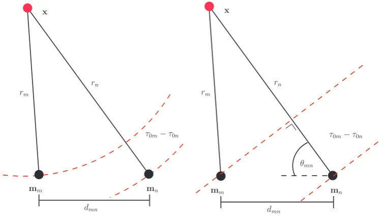
that time-delays are quoted in units of audio samples rather than seconds. Theℝ3 →ℝmapping deﬁned by equation 2.25 is referred to as the time-delay measurement function in this thesis. An illustration of the time-delay 𝜏𝑚𝑛 arising from two microphones is illustrated in ﬁgure2.1a.

For a given time-delay𝜏𝑚𝑛, the source positionxis constrained in 3𝐷space to a hyperboloid

of two sheets with focal points corresponding to the microphone positions m𝑚 and m𝑛. Several

techniques have been proposed for estimating the source position as the approximate intersec-tion of multiple hyperboloids corresponding to TDEs at multiple pairs of microphones [199]. Such approaches for TDE-based localisation can be complex, since ﬁnding the intersection is a nonlinear problem [192].

Furthermore, the hyperboloid deﬁned by a TDE at a pair of microphones is sensitive to slight changes in the estimated time-delay. As a result, the position estimate derived from the intersection of hyperboloids is normally equally sensitive to slight estimation errors. To address this issue, the localisation problem can be formulated as the solution to a set of intersecting spheres where the spheres are centred at the microphone locations [70]. This is popularly known in the literature as the spherical intersection method for source localisation.

(36)

the source position by considering it as residing at the centre of concentric spheres deﬁned by the source and microphone positions [7]. This concept is illustrated in ﬁgure2.2afor the 2𝐷case of concentric circles, however, it is easily formulated for application to the 3𝐷case of concentric spheres.

It is possible also, to approach the localisation task by simplifying the wave front model. When the distance between the source and the microphones is large relative to the distance between the microphones, the source is said to be in the far-field. In cases where this condition can be ascertained, the sound wave impinging on a pair of microphones can be assumed to be planar. In this case, a directional angle to the source relative to the microphones can be approximated using aTDE. This is shown in figure2.1b where under the far field assumption, theDOA of the source sound wave is approximated as

𝜃𝑛𝑚= cos−1 (

𝜏𝑚𝑛𝑐

𝑓𝑠𝑑𝑚𝑛 )

, (2.26)

where 𝑑𝑚𝑛 denotes the distance between the microphones. This is referred to in this thesis as

theDOA measurement function.

Localisation using the DOAmethod in the absence of TDE uncertainty is straightforward. The source location is simply determined as the intersection of bearing lines deﬁned through knowledge of the microphone positionsm𝑚 andm𝑛 and theDOAangles to a set of microphone

pairs. In the presence ofTDE uncertainty however, these bearing lines are unlikely to intersect at a single point. To account for such a situation, the closest intersecting points of all bearing line pair combinations can be determined and the source position estimate obtained as a weighted average of these points [113]. This localization strategy for the 2𝐷 case is illustrated in ﬁgure

2.2b. Extending this method to the 3𝐷 localisation problem is straightforward.

2.1.3.1 Time Delay Estimation

In order to employ TDE-based localisation it is necessary to estimate the relative time delay between multiple microphone pairs by some means. This thesis considers cross-correlation based time-delay estimation techniques which are the most straightforward and by far the most com-monly used in speaker tracking applications. The reader is referred to [85] and references therein for a review of existing time-delay estimation techniques.

In an attempt to reduce the effects of reverberation and noise on the source signal received at the microphones, it is normal practice to apply a pre-filter to the microphone outputs. If a pre-filterℎ𝑓𝑚(𝑡) is applied to the microphone signal𝑦𝑚(𝑡) then the processed microphone output

is given by,

𝑧𝑚(𝑡) =ℎ𝑓𝑚(𝑡)∗𝑦𝑚(𝑡). (2.27)

Under this assumed signal model, the cross-correlation of𝑧𝑚(𝑡) and𝑧𝑛(𝑡) can be used to estimate

(37)

m𝑚 m𝑛

x

𝜏0𝑚−𝜏0𝑛

𝑟𝑚

𝑟𝑛

𝑑𝑚𝑛

(a)Time-delay𝜏𝑚𝑛=𝜏0𝑚−𝜏0𝑛 between

mi-crophones m𝑚 and m𝑛 corresponding to a

spherical wave-front model.

m𝑚 m𝑛

x

𝜏0𝑚−𝜏0𝑛

𝑟𝑚

𝑟𝑛

𝜃𝑚𝑛

𝑑𝑚𝑛

(b)DOA 𝜃𝑚𝑛 between microphones m𝑚 and m𝑛 corresponding to the source position x.

TheDOAis deﬁned by the time-delay𝜏𝑚𝑛=

[image:37.595.127.507.116.330.2]

𝜏0𝑚−𝜏0𝑛under the planar wave-front model.

Figure 2.1: Illustration of the relative time delay and Direction Of Arrival (DOA) at a pair of microphones.

is deﬁned as,

𝑅𝑧𝑚𝑧𝑛(𝜏) =𝐸[𝑧𝑚(𝑡)𝑧𝑛(𝑡−𝜏)] (2.28)

where𝐸[⋅] denotes the expectation operator. The cross-correlation function attains a maximum at the relative time-shift between𝑧𝑚(𝑡) and𝑧𝑛(𝑡) where the correlation between the two signals

is greatest. The time-delay can therefore be estimated as,

ˆ

𝜏𝑚𝑛= arg max 𝜏

𝑅𝑧𝑚𝑧𝑛(𝜏). (2.29)

For two microphone signals 𝑧𝑚 and 𝑧𝑛 which are uncorrupted by noise or reverberation, the

maximum of equation 2.29is expected to occur at the true time delay𝜏𝑚𝑛=𝜏0𝑚−𝜏0𝑛. In real

(38)

m1 m2 m3 m4 m5 m6 x 𝜏12 𝜏34 𝜏56

(a)The source is located at the centre of a set of concentric circles where a single microphone is located on the circumference of a each circle [7].

m1 m2 m3 m4 m5 m6

x=𝑤1x1+𝑤2 x2+𝑤3x3

𝜃12 𝜃34 𝜃56 x1 x2 x3

(b) When the bearing lines to multiple micro-phone pairs do not intersect at a unique point, multiple possible source locations are obtained. In this example, the bearing lines deﬁned by the an-gles𝜃12,𝜃34,𝜃56intersect at locationsx1,x2and x3. When this occurs, a weighted sum ofx1,x2

and x3 can be used to estimate the true location

i.e.x=𝑤1x1+𝑤2x2+𝑤3x3. The weights𝑤1,𝑤2

and𝑤3 are determined based on the probabilities

of theTDEs used to estimate theDOA bearings

𝜃12,𝜃34,𝜃56[125].

Figure 2.2: Time-delay and DOAlocalisation techniques.

Generalised Cross-Correlation

Using the Wiener-Khintchine theorem, the cross correlation function of equation2.28 can also be represented as,

𝑅𝑧𝑚𝑧𝑛(𝜏) =ℱ−1{𝐸[𝑍𝑚(𝜔)𝑍𝑛∗(𝜔)]} (2.30)

where_ℱ−1_{⋅}is the inverse Fourier transform and the asterisk_∗denotes the complex conjugate. In terms of the applied pre-ﬁlters as in equation 2.27, the cross-correlation function is,

𝑅𝑧𝑚𝑧𝑛(𝜏) =

∫ _∞

−∞

𝐻𝑓𝑚(𝜔)𝐻𝑓∗𝑛(𝜔)𝐺𝑦𝑚𝑦𝑛(𝜔)𝑒

𝑗𝜔𝜏_𝑑𝜔 _(2.31)

=

∫ _∞

−∞

Ψ(𝜔)𝐺𝑦𝑚𝑦𝑛(𝜔)𝑒𝑗𝜔𝜏𝑑𝜔 (2.32)

where 𝐺𝑦𝑚𝑦𝑛(𝜔) is the cross-power spectrum of the unﬁltered microphone signals 𝑦𝑚(𝑡) and

𝑦𝑛(𝑡) and Ψ(𝜔) = 𝐻𝑓𝑚(𝜔)𝐻𝑓∗𝑛(𝜔) is the combined frequency domain weighting equivalent of

the time domain preﬁltersℎ𝑓𝑚(𝑡) and ℎ𝑓𝑛(𝑡). This is the Generalised Cross Correlation (GCC)

(39)

weighting functions Ψ(𝜔); also known as processors, rather than time domain pre-ﬁlters. For the case where Ψ(𝜔) = 1, this corresponds directly to cross-correlation without pre-ﬁltering.

Various frequency domain weighting functions exist for use withGCC, such as the Maximum Likelihood (ML) weighting [20],

Ψ𝑀 𝐿(𝜔) =

1

∣𝐺𝑦𝑚𝑦𝑛(𝜔)∣

∣𝛾𝑚𝑛∣2

[1_{− ∣}𝛾𝑚𝑛∣2]

. (2.33)

As can be seen from this, the ML processor acts to accentuate the signals at frequencies where the signal coherence is highest. This model is built on an anechoic (free space) sound propagation model with uncorrelated noise on the received signals. Therefore, the eﬀects of a reverberant environment on ML time-delay estimation, tends to reduce its accuracy and reliability consid-erably [12]. As a result it is not generally suitable in its basic form for speaker localisation in real room environments.

A more suitable processor which has found extensive use inTDE-based speaker localisation is the Phase Transform (PHAT) weighting [20],

Ψ𝑃 𝐻𝐴𝑇(𝜔) =

1

. (2.34)

The effect of this filter is to assign an equal weighting to the signals at each frequency. As a result, the correlation function obtained is determined using the phase information of the signals only. Since each frequency band is equally weighted however, errors are accentuated in frequency bands where the signal power is low [20]. Despite this, there is a strong theoretical basis [26,177] supporting the use of the PHATweighting above other processors in reverberant environments which is supported by empirical analysis [86]. Although the PHAT weighting is useful to counteract the effects of reverberation, it is not without its limitations and shows poor performance in low reverberant and low noise environments [88, Chapter 5].

As previously stated, the Generalized Cross-Correlation with Phase Transform (GCC-PHAT) weighting does not attempt to account for the presence of noise. To address this Wang et al. [75] proposed a modiﬁed form of the PHATprocessor to be applied as,

Ψ𝑀 𝑂𝐷_{𝑃 𝐻𝐴𝑇}(𝜔) = 1

𝛾_∣𝐺𝑦𝑚𝑦𝑛(𝜔)∣+ (1−𝛾)∣𝑁𝑚(𝜔)∣2

(2.35)

where 0≤𝛾 ≤1 is a weighting which is equivalent in its definition to the SRR. One difficulty inGCC weighting functions defined for background noise is that an estimate of the noise must be made. Typically, an estimate of background noise is made during periods when the source is not active.

(40)

indicate signal content which is largely unaﬀected by reverberation or noise. Their weighting aims to increase the contribution of such signal content in the correlation estimate and decrease that which deviates from this assumption. They employ a harmonic speech model and measure the deviation of the received microphone signals from this model to weight the signal content. The proposed weighting is deﬁned as,

Ψ𝑠=

(1₋𝑚𝑎𝑥[𝑒𝑚,𝑖, 𝑒𝑛,𝑖])𝛽

(2.36)

where𝑒𝑚,𝑖and𝑒𝑛,𝑖are the normalised errors between the𝑖th harmonic of the microphone signals

𝑚 and𝑛respectively, in relation to that deﬁned by the harmonic speech model. The variable𝛽

is a heuristically determined parameter and in the range𝛽 = [1,2]. Comparing, equation 2.34

and equation2.36it can be seen that Ψ𝑠is eﬀectively a weighted version of thePHATprocessor,

therefore it can observe similarly poor performance when the Signal to Noise Ratio (SNR) is low.

2.1.3.2 Fundamental Limitations on Time Delay Estimation

There is a fundamental limitation on the performance of time-delay estimation. The effect of the source signal properties which influence this performance limit can be characterised by the Cramér-Rao Lower Bound (CRLB). This performance measure defines a lower limit on the achievable variance of any unbiased TDE [6] and defines the uncertainty on the TDE locally about the true time-delay.

Assuming that the signal and noise spectra are constant for ₋2𝜋𝐵 _≤𝜔 _≤2𝜋𝐵 where 𝐵 is the signal bandwidth, then theCRLBon the variance of a time-delay estimate is given by [6,56],

𝜎_{𝐶𝑅𝐿𝐵}2 =

[

2𝑇

∫ 2𝜋𝐵

0

𝜔2

(

𝑆𝑁 𝑅2

1 + 2𝑆𝑁 𝑅

)

𝑑𝜔

]−1

(2.37)

= 3 8𝜋2

(1 + 2𝑆𝑁 𝑅)

𝑆𝑁 𝑅2

1

𝐵3_𝑇. (2.38)

It is clear that the assumption of constant signal power is unrealistic in speech applications. In the absence of a more speciﬁc treatment of the speech localisation problem in the available literature however, some insight into the expected performance of time-delay estimation can still be gained under this assumption.

(41)

these are related to the variance of a TDE in the following manner,

𝜎_{𝐶𝑅𝐿𝐵}2 _∝ 1

𝑆𝑁 𝑅2 (2.39a)

𝜎_{𝐶𝑅𝐿𝐵}2 _∝ 1

𝐵3 (2.39b)

𝜎_{𝐶𝑅𝐿𝐵}2 _∝ 1

𝑇 (2.39c)

Therefore, in designing a time-delay estimator, increasing any of these quantities improves the accuracy ofTDEs. In speech applications it is clear that the bandwidth𝐵is not under the control of the designer and is typically 3𝑘𝐻𝑧(400𝐻𝑧−3400𝑘𝐻𝑧). TheSNRhowever, generally decreases as the source-to-microphone distances increases. Therefore, ensuring that the microphones are close to the source can increase the SNR and improveTDEaccuracy. Also, increasing the time analysis window𝑇 will act to improve the accuracy ofTDEs. It is often the case however that𝑇

is dictated by the required measurement update rate. In tracking, typically the highest update rate is desired restricting 𝑇 to small values. A high update rate is therefore employed at the cost of reduced TDEaccuracy.

The CRLB, does not completely reflect the true nature of time-delay estimation perfor-mance as it incorporates noise analysis only and does not consider the effects of reverberation. As theSNRdecreases, a thresholding effect is observed whereby the accuracy of aTDEdiverges from that estimated by the CRLB. This is a result of the wrong peak in the cross-correlation function of equation2.29 being selected as that corresponding to the true time-delay estimate. This type of error arising due to anomalous TDEs is known as a “large” error in time-delay estimation problems and is not modelled by the CRLB. TheCRLBonly describes uncertainty locally about the true time-delay which is often referred to as a “small” error in the estima-tion problem. Considerable efforts have been made to theoretically model the performance of time-delay estimation in the presence of both large and small errors. Chapter 5 continues this discussion where these theoretical models are used in examining the localisation performance of a configuration of microphone arrays in a lecture room.

Improving the Reliability of Time Delay Estimates (TDEs)

Since reverberation can have such a signiﬁcant eﬀect on the accuracy and performance of TDE -based localisation, it can be useful to establish some measure of TDE reliability.

The most basic reliability measure is based on the energy of the microphone signals. Typi-cally, high signal energy will indicate the presence of a speech source. Only determining TDE

over frames of signiﬁcant energy can therefore yield more accurate estimates. More sophisti-cated approaches aim to directly classify the signal and speech or non-speech by learning the characteristic features of speech signals [44].

(42)

psyhcoacoustical phenomenon observed in humans where localisation is only performed on the direct sound wave. Employing the precedence effect in time-delay estimation requires firstly determining the onset of the direct sound wave in the microphone signals. Once this onset is determined, time-delay estimation is only applied over a short period at the detected onset [33]. By only considering a short period about the onset, time-delay estimation is not performed on the later arriving reverberations over which TDEs are less reliable. Additional techniques have examined modelling the precedence effect for localisation by learning the association of the spectral content of the microphone signals to that of localisation precision [108].

The value of the maximum peak in the GCC function and the ratio of the first and second largest peak can also be used to estimate TDE reliability. Typically, the value of the maxi-mum peak has a direct relation to the likelihood of it corresponding to a true sound source. Furthermore, the ratio of this peak value to that of the second largest peaks can also indicate its significance and therefore is reliability. Analysis of both these reliability criteria, has been shown to yield equivalent performance to that obtained by modelling the precedence effect [33]. Determining reliableTDEs can also be considered as an outlier estimation problem through some temporal based statistical analysis. Given a number of short temporal windows it is possible to build a histogram of the TDEs from which the true TDE can be determined as in [139]. Such an approach can be particularly useful in speech applications where the source signal is not always continuous but possibly intermittent.

2.1.4 Localisation through Sound Intensity Diﬀerences

Given the deﬁnition of sound intensity in2.1, it can be seen that it contains information relating to the distance to the source𝑟. If𝑃 is known, the distance to the sound source from a particular point could be determined simply by measuring the sound intensity at that point. In speaker localisation problems, 𝑃 is never known and not easily estimated. Furthermore, the inverse square law is a simple model of sound propagation and is not always adhered to, particularly if the omni-directional source model is violated.

In applications where the assumption of omni-directional sound propagation is valid, then a measure of the energy of the microphone signals can be used to localise an acoustic source. Consider an estimate of the energy of the 𝑚th microphone signal in equation2.16 obtained as,

𝐸𝑚 =

𝑎 𝑟_𝑖2

∫ 𝑇

0

𝑠2_𝑖(𝑡−𝜏0𝑚)𝑑𝑡+ ∫ 𝑇

0

𝑛2_𝑚_𝑚(𝑡)𝑑𝑡 (2.40)

=𝐸𝑠+ ∫ 𝑇

0

𝑛2_𝑚_𝑚(𝑡)𝑑𝑡, (2.41)

where𝐸𝑠is the source signal energy. It is assumed that the time analysis window𝑇 is suﬃciently

large such that the time-delay 𝜏0𝑚 does not aﬀect the signal energy estimates. Assuming for a

(43)

m𝑚 m𝑛

x

𝐸𝑚

𝐸𝑛

<

0

𝐸𝑚

𝐸𝑛

= 1

𝐸𝑚

𝐸𝑛

>

0

Figure 2.3: Localisation using interaural level diﬀerences.

variable, the following relationship between microphone signal energies can be deﬁned as [172],

𝐸𝑚

𝐸𝑛

= 𝑟

2

𝑛

𝑟2_𝑚 (2.42)

This relationship constrains the position of the sound source to a surface in 3𝐷 space as illus-trated in ﬁgure2.3. The intersection of the 3𝐷surfaces deﬁned by multiple pairs of microphones using this relation can then be used in localising the position of the source.

The successful use of interaural level diﬀerences for localisation requires the direct measure-ment of the source signal energy using multiple microphones. If the microphone signals are distorted due to reverberation or noise, this is generally not possible. As a result, techniques which use interaural level diﬀerences for localisation have found little use in real room environ-ments. Furthermore, the assumption of an omnidirectional source is generally too restricting for the speaker localisation task.

2.1.5 Steered Response Power based Localisation

Steered Response Power based localisation methods search a number of hypothesised speaker locations for the position corresponding to the maximum received power at the microphones. For each location under examination, a steering vector is deﬁned to steer an array of microphones to that position. A measure of the total received power from that position can then be used to clarify as to whether or not the position corresponds to an active speaker.

Given the observed vector of signals in equation2.21, we can aim to recover the source signal

(44)

as,

D𝐻(𝜔)Y(𝜔) =D𝐻(𝜔)𝑆(𝜔)D(𝜔) +D𝐻(𝜔)N𝑚(𝜔) (2.43)

=𝑆(𝜔) +D𝐻(𝜔)N𝑚(𝜔) (2.44)

The operation on the observation vectorY(𝜔) in equation2.43can be thought of as time aligning the microphone output signals and determining their weighted sum. This is known as thedelay and sum beamformer. The success of the delay-and-sum beamformer relies on the source signals to sum coherently and the noise and reverberant signal components to sum incoherently.

Since the steering vector is dependent on the source positionxthe beamformer can be steered to any hypothesised position. Using the audio-based measurement function of equation2.25the expected time delay corresponding to a hypothesised source positionxcan be determined. These expected time-delays can then be used to deﬁne a steering vector ˆD(𝜔,x). Throug