Optimisation of material properties for the modelling of large deformation manufacturing processes using a finite element model of the Gleeble compression test

Optimisation of material properties for the

modelling of large deformation manufacturing

processes using a finite element model of the

Gleeble compression test

C.J. Bennett, W. Sun

Department of Mechanical,

Materials and Manufacturing Engineering,

University of Nottingham,

Nottingham NG7 2RD, UK

Abstract

1

Introduction

Finite Element (FE) modelling of large deformation manufacturing processes such as forging, forming, welding and machining requires a wide range of ma-terial properties to be generated in order to represent the mama-terial behaviour. The relevant plastic flow stress data is usually generated across a wide range of temperatures and strain rates by using axisymmetric compression testing. Typically isothermal compression tests are used, where specimens are soaked at the test temperature to remove the temperature gradient from within the specimen before the compression test is performed [?], however this soak time can significantly alter the microstructure of the material meaning that the test does not represent the condition of the material during the actual pro-cess. An alternative method is a compression test following rapid heating, such as that used in the Gleeble thermo-mechanical simulator. The Gleeble uses the resistance heating method to achieve high heating rates and once the test temperature is reached at the desired heating rate, the compression test is then performed.

Conventional material testing methods can be used to determine basic material properties accurately (such as Young’s modulus for example). How-ever with more complex testing methods such as thermo-mechanical com-pression testing, additional effects such as an initial specimen temperature profile, adiabatic heating or the effects of friction can influence the output of the test making the results more difficult to interpret [?, ?, ?, ?]. Opti-misation techniques are one tool that can be used to improve the quality of material data generated for use in FE modelling.

Optimisation of the elastic-plastic properties of a power-law material us-ing data from both the loadus-ing and unloadus-ing curves generated durus-ing in-dentation testing of materials was carried out by Kang et al. [?, ?]. They produced both axisymmetric and 3D FE models of the indentation tests us-ing the ABAQUS FE software and a routine developed usus-ing the MATLAB programming environment to perform the optimisation. They concluded that the results of the optimisation were significantly improved when con-sidering multiple indenters of different geometries and that the accuracy of the optimisation was reduced when considering the optimisation of material parameters using experimental curves as opposed to target datasets created from known parameters using the FE model.

Oldenburg [?], however this model did not include the effects of an initial temperature profile present within the specimen or adiabatic heating dur-ing the compression, which could lead to errors in the optimised results as highlighted by the work of Bennett et al. [?, ?].

The focus of this work is to develop a robust optimisation procedure that can be used to improve the characterisation of the large deformation plastic behaviour of materials, in the form of a Norton-Hoff material model in this case, using experimental Gleeble compression data and an FE model of the Gleeble compression process. The Norton-Hoff material model is often used to represent large strain plastic flow stress of a material across a wide range of temperatures and strain rates [?], which is particularly applicable for the modelling of forming and forging manufacturing processes [?,?, ?]. The FE model included in this optimisation process includes the resistance heating of the specimen and the adiabatic heating during compression, which have both been shown to be important and can affect the flow stress data which is generated during the test [?].

2

Finite Element Gleeble compression test

model

A Finite Element (FE) model of the Gleeble compression test model, which has been developed in the DEFORM FE software [?], is used in this work to form the basis for optimisation of the material properties. An overview of this model is presented in Figure 1.

The maximum specimen diameter from the FE model is used to derive the strain, ε, according to:

ε= 2ln

_D

0+ ∆D

D0

(1)

and stress, σ, according to:

σ = _π(D F

0+∆D)2 4

(2)

whereD0 is the original specimen diameter, ∆Dis the change in specimen

The frictional shear stress,fs, between the platens and specimen is

com-monly represented using one of the following two relationships:

fs =µp (3)

wherepis a compressive normal stress andµis the coefficient of friction, or:

fs =mk (4)

where m is the friction coefficient and k is the shear strength of the material.

Equation ?? is commonly used to the represent the friction shear stress during sheet metal forming, while Equation ?? is commonly used in the analysis of bulk metal forming such as that discussed in this work [?]. As such a value of 0.3 is used for m in Equation ?? throughout the analyses in this work as it was shown in the work of Bennett et al. [?] that the results are relatively insensitive to this value.

2.1

Test parameters

In this work, two test temperatures and two nominal strain rates have been chosen as the basis for the optimisation procedure. Initial temperature fields in the specimen have been generated at 900◦C and 1100◦C using the tech-niques described by Bennett et al. [?]. Strain rates of 1 and 10 s−1 are considered.

2.2

Material Model

For Nickel-based superalloys, typically there is no reduction in yield strength below around 800◦C due to the strengthening phases that exist in the ma-terial [?]. Above around 800◦C, these strengthening phases begin to dissolve and the yield strength reduces. In this temperature region (T >0.5Tm, where

Tmis the melting temperature) and at large deformations, as considered here,

the behaviour of the material is strongly dependent on the strain rate [?] and therefore the equivalent flow stress of the material, ¯σ can be represented by the Norton-Hoff material model of the form:

¯

σ =K(¯ε+ ¯ε0)nε˙¯

m β

Tabs

!

where ¯ε is the equivalent plastic strain,K (MPa sm_{), m, n, ¯ε}

0 and β (K)

are material constants and Tabs is the absolute temperature in Kelvin.

The experimental Gleeble compression data for the material used as a basis for this study at 900◦C and 1100◦C is presented in Figure 2. It can be seen that significant softening of the material occurs over this temperature range, with peak stresses shown at approximately 1300 MPa at 900◦C at a nominal test rate of 10 s−1_{, reducing to under 400 MPa at 1100}◦_{C at the}

same rate.

3

An optimisation procedure for determining

material properties

3.1

Optimisation model

In this study, a non-linear optimisation technique has been devised within the MATLAB programming environment using the non-linear least-squares optimisation function (LSQNONLIN) [?].

This optimisation procedure is guided by the gradient evaluation and iterates until convergence is reached. The optimisation model in this work is:

F(x) =

n

X

i=1

[σ(x)pre_i −σ_itarget]2 →min (6)

where F(x) is the objective function, x is the optimisation variable,

σ(x)pre_i is the predicted stress from the finite element model and σ_itarget is the target stress data at a corresponding strain level, denoted by the data-point i and n is the number of test data pairs.

x is a vector in the n-dimensional space, Rn, which contains the set of material constants in the Norton-Hoff model

x∈Rn (7)

x= [K, m, n,ε¯0, β]T (8)

where LB and U B are the lower and upper bounds respectively of x

during the optimisation as presented in Table ??.

Table 1: Lower and upper bounds of x

Parameter LB UB

K 0 0.2

m 0 0.5

n 0 0.5

¯

ε0 0 0.1

β 0 20000

3.2

Optimisation procedure

The outline of the optimisation procedure is defined in Figure 3. Initial values of the material constants are provided and a series of functions have been written in MATLAB to control the pre-processing, post-processing and running of the DEFORM Finite Element (FE) compression models during the optimisation process. A set of base key-files for the compression models containing test conditions including the initial temperature field are held throughout the optimisation process, which are modified on each call of the objective function with the appropriate Norton-Hoff material constants to define the behaviour of the material.

Load and radial displacement data at the axial centre on the surface of the specimen are extracted from each of the DEFORM Gleeble compression models and converted to stress-strain curves (according to Equations ??and

??) to compare with the target values (either experimental or a reference model). Each function call results in four FE models being run to generate a complete dataset of stress-strain values across the range of test conditions for each new set of material constants. The history of the optimisation process is recorded by storing the material constants at each iteration in an external file using a custom output function called by the LSQNONLIN function.

4

Optimisation using reference stress-strain

curves from Finite Element simulation

values is then chosen for the optimisation process and the convergence of the solution is checked against the target solution and values. This process is performed for a reduced, three parameter version of the Norton-Hoff mate-rial model (Equation ??) and the full five parameter model as presented in Equation ??.

4.1

Three parameter optimisation

Initial trials were carried out using a reduced three parameter material model. The values ofnand ¯ε0 in Equation??were set to 0, removing the dependency

on strain and reducing the material model to:

¯

σ=Kε˙¯m β

Tabs

!

(10)

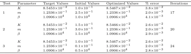
The target stress-strain curves (σ_itarget) were generated using material constants derived from a least-squares fit of Equation??to the experimental data. Three sets of initial guess parameters (test 1, test 2 and test 3) were then chosen and the convergence of the solutions is presented in Figure 4 along with the details of the optimisation results in Table ??. These results show that the errors in the constants produced by the optimisation procedure are very low (less than 1×10−1 _{% in all cases) for the three parameter model}

and verifies the validation procedure that has been developed.

Table 2: Three parameter optimisation

Test Parameter Target Values Initial Values Optimized Values % error Iterations

K 8.5453×10−2 1.0×10−1 8.5467×10−2 3.8×10−2 1 m 1.2336×10−1 2.5×10−1 1.2336×10−1 2.0×10−3 17

β 1.0906×104 1.0×104 1.0906×104 4.1×10−3

K 8.5453×10−2 1.5×10−1 8.5466×10−2 2.6×10−2 2 m 1.2336×10−1 3.0×10−1 1.2336×10−1 2.0×10−3 20

β 1.0906×104 1.5×104 1.0906×104 2.9×10−3

K 8.5453×10−2 _1.0×10−1 _8.5467×10−2 _2.6×10−2

3 m 1.2336×10−1 _0.1×10−1 _1.2336×10−1 _2.0×10−3 ₂₄ β 1.0906×104 0.5×104 1.0906×104 2.8×10−3

4.2

Five parameter optimisation

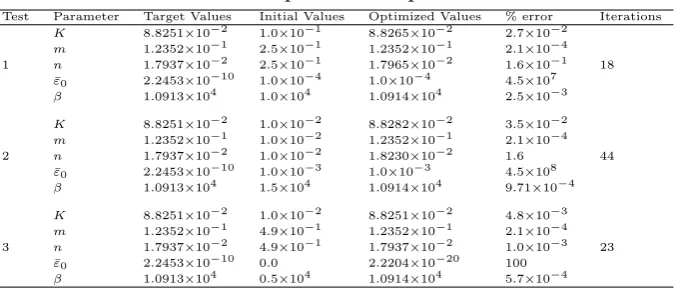
were chosen to verify the optimisation procedure. These initial parameters, along with the target and final optimised values, are presented in Table ??. It can be seen in all cases for the five parameter material model that the number of iterations required to determine the optimised material properties are considerably more than with the three parameter material model due to the increased complexity of the problem. For this model, the errors in the constantsK,m,nandβ are all less than 2% however large errors are present in the value of ¯ε0 that has been determined, however, as Figure 5 shows for

the example of 900◦C at 1 s−1, the Norton-Hoff material model is insensitive to the value of ¯ε0 at the high plastic strain values considered in this work,

showing only sensitivity below strain values of approximately 2×10−3_.

Table 3: Five parameter optimisation

Test Parameter Target Values Initial Values Optimized Values % error Iterations

K 8.8251×10−2 _1.0×10−1 _8.8265×10−2 _2.7×10−2 m 1.2352×10−1 _2.5×10−1 _1.2352×10−1 _2.1×10−4

1 n 1.7937×10−2 2.5×10−1 1.7965×10−2 1.6×10−1 18 ¯

ε0 2.2453×10−10 1.0×10−4 1.0×10−4 4.5×107 β 1.0913×104 1.0×104 1.0914×104 2.5×10−3

K 8.8251×10−2 1.0×10−2 8.8282×10−2 3.5×10−2

m 1.2352×10−1 1.0×10−2 1.2352×10−1 2.1×10−4 2 n 1.7937×10−2 1.0×10−2 1.8230×10−2 1.6 44

¯

ε0 2.2453×10−10 1.0×10−3 1.0×10−3 4.5×108 β 1.0913×104 _1.5×104 _1.0914×104 _9.71×10−4

K 8.8251×10−2 1.0×10−2 8.8251×10−2 4.8×10−3

m 1.2352×10−1 4.9×10−1 1.2352×10−1 2.1×10−4 3 n 1.7937×10−2 4.9×10−1 1.7937×10−2 1.0×10−3 23

¯

ε0 2.2453×10−10 0.0 2.2204×10−20 100 β 1.0913×104 0.5×104 1.0914×104 5.7×10−4

The convergence history of the remaining four parameters is presented in Figure 6, which again shows good convergence from a wide range of initial parameters.

5

Optimisation using experimental stress-strain

curves

the ability of the optimisation process to determine material constants from a non-related initial set of values. The optimisation process used Gleeble compression models run across the same range of parameters used in the experimental testing (at 900 and 1100◦C with nominal strain rates of 1 and 10s−1_).

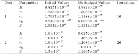
The results of the optimisation process are presented in Table ?? for both of the tests, while the optimisation history is shown in Figure 7. It can be seen that, as expected, the optimisation process is complete in fewer iterations for Test 1 when the initial constants have been determined from the experimental data. The percentage difference between the two tests carried out using the experimental target data is presented in Table ??where it can be seen that while differences appear between the coefficients determined from the optimisation procedure, they are less than 10% in all cases showing that the optimisation procedure is robust enough to cope with an arbitrary guess of initial constants.

A comparison is made between the experimental Gleeble compression data and the Gleeble compression model run with both the original and optimised Norton-Hoff parameters from Test 1 in Figure 8. A significant improvement can be seen in the correlation of the Gleeble model data run with the optimised parameters, particularly at the lower temperature (higher stress values), suggesting that they are a better representation of the actual behaviour of the material.

Table 4: Five parameter optimisation using experimental target data

Test Parameter Initial Values Optimized Values Iterations

K 8.8251×10−2 4.9829×10−2

m 1.2352×10−1 1.5036×10−1 1 n 1.7937×10−2 1.1188×10−2 16

¯

ε0 2.2453×10−10 6.8898×10−11

β 1.0913×104 _1.1913×104

K 1.0×10−2 5.0276×10−2

m 1.0×10−2 1.4669×10−1 2 n 1.0×10−2 1.2086×10−2 26

¯

ε0 1.0×10−3 1.0×10−3 β 1.5×104 _1.1907×104

Table 5: Percentage difference between Test 1 and 2 optimised values

Parameter Percentage difference between test 1 and 2 values

K 0.89

m 2.5

n 7.7

¯

ε0 not applicable

6

Conclusions

An optimisation procedure has been developed and implemented in MAT-LAB using a Finite Element (FE) model of the Gleeble compression test, which includes the initial temperature profile in the specimen and adiabatic heating, in order to optimise the five parameters (K, m, n, ¯ε0 and β) of the

Norton-Hoff material model. The optimisation algorithm developed has been shown capable of optimising the parameters to within 1% of a set of target values using various initial guess values based on a simplified three parame-ter maparame-terial model. When the five parameparame-ter maparame-terial model was considered, good convergence to the target values were shown (to within 10%) for four out of the five parameters and poor convergence was shown for the ¯ε0

param-eter, however, it was shown that the dominant behaviour of this parameter was at low strain values which were not the main focus of this study. It is expected however that similar convergence could be achieved for this value if small strain behaviour was being considered.

A significant improvement in the stress-strain curves generated from the Gleeble compression model was shown when the optimisation process was carried out for two initial parameter sets using the experimental stress-strain data as the target curves for the optimisation. This suggests that the opti-misation procedure, coupled with the Gleeble compression model could be used to improve the representation of materials for other forming and forg-ing modellforg-ing applications where accurate material data is key to generatforg-ing useful results.

Acknowledgements

The authors wish to thank Rolls-Royce plc, Aerospace Group, for their fi-nancial support of the research, which was carried out at the University Technology Centre in Gas Turbine Transmission Systems at the University of Nottingham. The views expressed in this paper are those of the authors and not necessarily those of Rolls-Royce plc, Aerospace Group.

References

tests. NPL good practice guide no. 3. Technical report, National Physical Laboratory, 1997.

[2] R.W. Evans and P.J. Scharning. Axisymmetric compression test and hot working properties of alloys. Materials Science and Technology, 17(8):995–1004, 2001.

[3] R.W. Evans and P.J. Scharning. Strain inhomogeneity in hot ax-isymmetric compression test. Materials Science and Technology, 18(11):1389–1398, 2002.

[4] C.J. Bennett, S.B. Leen, E.J. Williams, P.H. Shipway, and T.H. Hyde. A critical analysis of plastic flow behaviour in axisymmetric isothermal and gleeble compression testing. Computational Materials Science, 50(1):125 – 137, 2010.

[5] C.J. Bennett, S.B. Leen, and P.H. Shipway. A finite element analysis of errors in axisymmetric isothermal and gleeble compression testing of Ti-6Al-4V. International Journal of Material Forming, 3:1155–1158, 2010.

[6] J.J Kang, A.A Becker, and W Sun. A combined dimensional analy-sis and optimization approach for determining elasticplastic properties from indentation tests. The Journal of Strain Analysis for Engineering Design, 46(8):749–759, 2011.

[7] J.J. Kang, A.A. Becker, and W. Sun. Determining elasticplastic prop-erties from indentation data obtained from finite element simulations and experimental results. International Journal of Mechanical Sciences, 62(1):34 – 46, 2012.

[8] P. ˚Akerstr¨om and M. Oldenburg. Studies of the thermo-mechanical material response of a boron steel by inverse modelling. J. Phys. IV France, 120:625–633, 2004.

[9] J.-L. Chenot and F. Bay. An overview of numerical modelling techniques.

Journal of Materials Processing Technology, 80-81(0):8–15, 1998.

Technology, 157-158(0):131 – 137, 2004. Achievements in Mechanical and Materials Engineering Conference.

[11] X. Duan and T. Sheppard. The influence of the constitutive equation on the simulation of a hot rolling process. Journal of Materials Processing Technology, 150(12):100 – 106, 2004.

[12] C.J. Bennett. A comparison of material models for the numerical simu-lation of spike-forging of a CrMoV alloy steel. Computational Materials Science, 70(0):114 – 122, 2013.

[13] S. Kobayashi, S.I. Oh, T. Altan. Metal Forming and the Finite-Element Method, 1st Ed. New York: Oxford University Press, 1989.

[14] R. Reed. Superalloys, 1st Ed. Cambridge: Cambridge University Press, 2006

[15] A. Moal, E. Massoni. and J.L. ChenotA Finite element modelling for the inertia welding process. in Proc. of Int. Conf. on Computational Plas-ticity (eds D.R.J. Owen, E. Onate and E. Hinton,), Barcelona, Spain, 6th-10th April 1992, Swansea: Pineridge Press