The multi thermal and multi stranded nature of coronal rain

THE MULTI-THERMAL AND MULTI-STRANDED NATURE OF CORONAL RAIN

P. Antolin1, G. Vissers2, T. M. D. Pereira2, L. Rouppe van der Voort2, and E. Scullion3

1

National Astronomical Observatory of Japan, Osawa, Mitaka, Tokyo 181-8588, Japan;[email protected]

2

Institute of Theoretical Astrophysics, University of Oslo, P.O. Box 1029, Blindern, NO-0315 Oslo, Norway

3

Trinity College Dublin, College Green, Dublin 2, Ireland

Received 2015 February 2; accepted 2015 April 16; published 2015 June 9

ABSTRACT

We analyze coordinated observations of coronal rain in loops, spanning chromospheric, transition region(TR), and coronal temperatures with sub-arcsecond spatial resolution. Coronal rain is found to be a highly multithermal phenomenon with a high degree of co-spatiality in the multi-wavelength emission. EUV darkening and quasi-periodic intensity variations are found to be strongly correlated with coronal rain showers. Progressive cooling of coronal rain is observed, leading to a height dependence of the emission. A fast-slow two-step catastrophic cooling progression is found, which may reflect the transition to optically thick plasma states. The intermittent and clumpy appearance of coronal rain at coronal heights becomes more continuous and persistent at chromospheric heights just before impact, mainly due to a funnel effect from the observed expansion of the magneticfield. Strong density inhomogeneities of0. 2 0. 5″ − ″ are found, in which a transition from temperatures of 105to 104K occurs. The0. 2″ – 0. 8″ width of the distribution of coronal rain is found to be independent of temperature. The sharp increase in the number of clumps at the coolest temperatures, especially at higher resolution, suggests that the bulk distribution of the rain remains undetected. Rain clumps appear organized in strands in both chromospheric and TR temperatures. We furtherfind structure reminiscent of the magnetohydrodynamic(MHD)thermal mode(also known as entropy mode), thereby suggesting an important role of thermal instability in shaping the basic loop substructure. Rain core densities are estimated to vary between 2 × 1010and2.5×1011cm−3, leading to significant downward massfluxes per loop of 1–5 × 109g s−1, thus suggesting a major role in the chromosphere-corona mass cycle.

Key words:instabilities– magnetohydrodynamics(MHD)–Sun: activity– Sun: corona– Sun:filaments, prominences–waves

Supporting material:animations

1. INTRODUCTION

The solar corona, the outermost layer of the solar atmo-sphere, has an average temperature above a million degrees, a fact that has puzzled astrophysicists for decades. The processes responsible for this heating are still unknown, mostly due to the very short time and spatial scales on which they operate. However, not everything in the corona is hot. Structures at chromospheric temperatures are clearly present in the solar corona. Evidence for this has been found for more than a century, since the first detection of prominences in the solar atmosphere (Secchi1875). In the last 40 yr, especially in the last few years with the advent of high-resolution instruments, smaller chromospheric structures with a more pervasive character have been shown to occur intermittently in the corona above active regions (Kawaguchi 1970; Leroy 1972; Schrijver 2001; Antolin & Rouppe van der Voort 2012; Antolin et al.2012; Ahn et al.2014). This material is known as coronal rain: partially ionized, dense clumpy structures catastrophically cooling in the corona and accreting toward the solar surface. Its occurrence is considered as the direct observational consequence of the thermal instability mechan-ism, in which radiative losses locally overcome the heating processes.

The presence of prominences in the corona and especially the recent detection of coronal rain with a more pervasive character entails fundamental aspects of the interaction of plasmas and fields in low β environment in which thermal instability plays a central role. This mechanism is intrinsically linked to the characteristic cooling aspects of the heating

mechanisms and provides far less strict detection possibilities due to the longer timescales and an enormous gain in spatial resolution when observing in wavelengths associated with cool emission. The study of coronal heating through associated cooling therefore provides unique advantages.

A big unknown in the physics of the solar corona is what percentage of coronal plasma is thermally unstable. This is also of significant importance for stellar coronae, since high-speed accretion of chromospheric plasma can produce characteristic profiles in their UV and optical range spectra, both from the falling plasma and from the impact into the lower atmosphere

active region loop to undergo catastrophic cooling. Based on Hαdata from the CRisp Imaging SpectroPolarimeter(CRISP) instrument at the Swedish 1-m Solar Telescope(SST), Antolin & Rouppe van der Voort(2012, hereafter Paper I)reduced the occurrence frequency to half a day or less, and estimated the coronal rain mass flux to be about one-third of that uploaded into the corona from spicules, thus stressing an important role in the chromosphere-corona mass cycle.

Paper Ipredicted that most of the rain material may pass undetected in coarse resolution instruments due to average clump4 widths of 300 km (and lengths of 700 km or so). Condensations were reported to be clustered in space into groups of correlated events, which indicates that the properties of coronal heating can be correlated over a significant spatial scale and that individual strands (the theoretical internal components of coronal loops)are not necessarily uncorrelated in their evolution. However, while most condensations were found to be correlated in time, only a few events, termed “showers”inPaper I, were found to occur close enough, which would produce large enough EUV absorption detectable with the coarser resolution of coronal instruments. Still, the limit cycles that thermally unstable loops experience, predicted from numerical simulations, should be visible observationally as periodic variations of the EUV intensity(which would then be correlated to the appearance of coronal rain). Such behavior has recently been reported and seems tofit well into the thermal non-equilibrium scenario (Froment et al.2015).

Since it is chromospheric (cool) plasma occurring in the corona, coronal rain constitutes the highest resolution window into the substructure of loops, and provides a tool for revealing the global magneticfield topology. First evidence for this was provided inPaper I, where the tracking of rain over a decaying active region allowed us to calculate the fall angle of the clumps, and therefore to reveal the large-scale morphology of the magnetic field and distinguish several loop families by tracing the clumps along the legs. The coronal rain condensa-tions were reported to be organized locally as strand-like structure with average widths around 300 km and lengths around 700 km, with nonetheless broad distributions down to 100 and 200 km, and up to 700 and 2400 km, respectively, for widths and lengths. The multi-strand substructure of loops was also reported in on-diskobservations of coronal rain with CRISP in Antolin et al.(2012)and more recently in Scullion et al. (2014). The latter work extends such findings to the coronal rain produced in post-flare loops and to the apexes of loops. In that work the distribution of widths peaks at 100 km, clearly indicating that the bulk of the distribution is unresolved due to the lack of resolution. Interestingly, the lengths of some of the observed condensations were reported to span up to 26,000 km, further underlining the global coronal magnetic field tracing possibilities offered by coronal rain.

The strand-like structure revealed by coronal rain along loops appears similar to the thread-like structure observed in prominences of certain types(e.g., active region prominences, Okamoto et al.2007). A relevant question is therefore whether such structure is strongly dependent on thermal instability, or whether such structure also exists at coronal temperatures under equilibrium conditions, in accordance with the debated multi-strand scenario in loops (Klimchuk 2006; Brooks et al. 2012, 2013; Peter et al. 2013). The loss of pressure

produced by thermal instability produces local accumulation of material leading to condensations. Given a thermally unstable loop, the continuous occurrence in the same spot of thermal instability, combined with the produced strongflows(or other possible siphon flows) in a low β environment such as the corona can easily lead to strand-like structure, as shown in multidimensional MHD simulations(Fang et al.2013). In this paper we show that even in this scenario it is reasonable to expect that such strand-like structure is not locally confined to the thermally unstable regions (and thus only confined to the low-temperature plasma in the loop), but extends along the entire loop and therefore to the hot coronal plasma as well. Therefore, even if a loop does not tend to be originally multi-stranded, it is possible that such organization is attained due to thermal instability and maintained thereafter. Such a scenario, for which we provide support in this paper(also theoretically supported by Low et al.2012b), has not been considered before and may significantly impact on the evolution of the coronal loop.

It can therefore be expected that a multithermal structure accompanies a multi-strand organization of the plasma in thermally unstable loops. This is shown in Scullion et al.

(2014), where loops observed in the coronalfilters of AIA are co-spatial with the Hαcondensations. The lack of resolution of AIA unfortunately does not allow us to see the details and spatial scales at which such multithermality can exist. In this work, with the help of the high resolution of the Interface Region Imaging Spectrograph(IRIS), we extend this result.

We present two data sets that combine multi-wavelength instruments spanning chromospheric, transition region (TR) and coronal temperatures. SST/CRISP,Hinode/SOT, IRIS/Slit-Jaw Imaging (SJI) and Solar Dynamics Observatory (SDO)/ AIA are used to reveal the multi-strand and multithermal aspects of coronal rain at unprecedented detail. The paper is organized as follows. In Section 2 the observations are presented. In Sections3and4the temperature and morphology of the observed condensations are presented, respectively. Results are discussed in Section5and conclusions are given in Section6.

2. OBSERVATIONS

2.1. Data Processing

In this work we analyze two different data sets correspond-ing to solar limb observations above active regions. The first data set combines data from SST(Scharmer et al.2003a)with the CRISP spectropolarimeter and the AIA instrument(Lemen et al.2011)ofSDO, dates from 26 June 2010 from 10:03 UT to 11:40 UT, and was centered on AR 11084 at [ , ]x y = [ 875,− −319]. The second data set, which combines the SOT telescope on board Hinode (Tsuneta et al. 2008), the SJI instrument of IRIS (de Pontieu et al. 2014) and SDO/AIA, dates from 2013 November 29 from 22:30 UT to 23:30 UT and wasfocused on AR 11903. IRIS/SJI was centered at

x y

[ , ]=[944,−264] fully containing the Hinode/SOT field of view(FOV), centered at[ , ]x y = [959,−220]. The context images for these coordinated observations are presented in Figures 1 and 2, where different colors denote different wavelengths, and the different FOV of each instrument can be compared.

We mainly focused on the SDO/AIA filters 304, 171, and 193, corresponding to a range of TR to coronal temperatures 4

usually spanned by thermally unstable plasmas. The upper photospheric filters 1600 and 1700 were also used for co-alignment purposes (see Section 2.2). Level 1.5 data from the SDO/AIA was used, obtained through the normal calibration routines in SolarSoft. Full diskimages are provided from AIA with a cadence of 12 s, an image scale pixel of 0″. 6 pixel−1, and a spatial resolution of 1″. 3–1″. 7.

IRIS combines anSJI and a spectrograph (SG). The IRIS data used here comprises only the SJI instrument since theIRIS slit was not located on the region of interest. Therefore, in this work only the coronal rain imaging capabilities of IRIS are shown. The data set corresponds to level 2 data from a

sit-and-stare observation combining the SJI 1400, 1330, and 2796 filters, dominated respectively by the SiIV TR lines 1393.78

and 1402.77 Å(formed around logT =4.8), the CII

chromo-spheric lines 1334.53 and 1335.71 Å(formed around

T

log =4.3), and the MgII k chromospheric line 2796.35 Å (formed around logT=4). IRIS/SJI provides an FOV of

175″ ×175″, an image scale pixel of 0″. 166 pixel−1 and a spatial resolution of 0″. 33(for the FUV)−0″. 4(for the NUV). The cadence for this observation is 36.5 s in eachfilter.

CRISP (Scharmer et al. 2008) at SST sampled the Hα spectral line at 41 line positions with 0.085 Å steps

(3.9 km s−1), in the spectral window [−1.7, 1.7]Å(≃ ±78

km s−1)with a cadence of 9 s. The FOV of SST for the present observation is53″ ×57″. The images benefited from the SST adaptive optics system(Scharmer et al.2003b)and the image restoration technique Multi-Object Multi-Frame Blind Decon-volution (van Noort et al. 2005). Although the observations suffered from seeing effects, most of the images are close to the theoretical diffraction limit for SST at the wavelength of Hα:

D 0. 14

λ ≃ ″ . We employed the same reduction procedure as in Paper I, which used early versions of parts of the data pipeline CRISPRED(de la Cruz Rodríguez et al.2015).

Hinode/SOT recorded filtergrams in the CaII H band (formed aroundlogT =4)at a cadence of 4.8 s. The image scale pixel is 0″. 109 pixel−1 and the spatial resolution is

D 0. 2

λ ≃ ″ . The SOT FOV for this observation is55. 8″ × 55. 8″ . Processing of data was carried out through the normal calibration routines in SolarSoft.

2.2. Co-alignment Procedures

The co-alignment of SST/CRISP andSDO/AIA data for the 2010 June 26 first consisted of determining the solar-x y

coordinates and locatingthe solar north direction for each CRISP frame. We then eliminated the SST drift byfixing each frame on the sunspot of AR 11084, at the center of the SST FOV, to reduce the frame-to-frame motion of the loop’s footpoints (and therefore of the loops themselves). The location of the solar limb for each frame was also determined, which allowed us to apply a gradient filter, reducing the intensity of on-diskfeatures for better visualization of the off-limb structures.SDOdata was then cropped and interpolated to the exact SST FOV. Small misalignments still remain, which are then corrected through cross-correlation using photospheric bright points (with long enough lifetime) and the solar limb location(using the AIAfilters 1600 and 1700, in combination with the far wing positions of Hα, which mostly show the photosphere).

For the SOT–SJI–AIA co-alignment, wefirst removed the slow drift of SOT by co-alignment of the images through tracking the movement of the limb. The cumulative offsets from this drift were applied to the time series, resulting in a rigid co-alignment on the order of one pixel or less. TheIRIS/ SJI images do not have this slow drift, but occasional wobble shifted the images a few pixels(this is normal during eclipse season). Such shifts were measured by applying cross-correlation techniques and applied to the time series. Then, to co-align the images from different instruments the following procedure was used. First, the AIA images were co-aligned and cropped to the SJI FOV by identifying common bright points in the AIA 1600 filter and the SJI 1400 filter. Afterward, both AIA and SJI images were interpolated to SOT’s image pixel

Figure 1.Composite image fromSDO/AIA combining three AIAfilters, 193 (red), 171(green), and 304(blue), showing data set 1: AR 11903 at the east limb on 2010 June 26. The dotted square denotes thefield of view of Figure3. The dotted loop corresponds to loop 2 studied in Section 3.2. The dashed square denotes thefield of view of SST.

(An animation of thisfigure is available.)

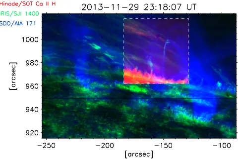
Figure 2.Composite image combining AIA 171(blue),IRIS/SJI 1400(green), andHinode/SOT CaIIH(red), showing data set 2: AR 11903 at the West limb

on the 2013 November 29. The dashed square denotes thefield of view covered by Hinode/SOT. The loop with coronal rain toward the center right of the square corresponds to the loop studied in this data set.

scale and were co-aligned using common features on the SJI 1400filter and SOT’s CaIIHfilter.

2.3. Methods

Due to the complex interplay of forces in loops coronal rain dynamics can be extremely complex, especially when obser-ving at sub-arcsecond resolution. Furthermore, their thermo-dynamic state is also expected to change, as we show in this paper, and as has been also indicated in Harra et al.(2014). A consequence of this is that it is very difficult to follow a single rain clump(at high resolution)over long distances. The clumps will usually split, merge, and elongate along their paths. For these reasons, especially for the CRISP data where myriads of small clumps are observed and for which the line-of-sight

(LOS)superposition is significant, individual tracking is very difficult and time consuming. For automatically detecting rain in the CRISP data we have therefore opted for perpendicular cuts across the loops at positions where rain is observed, rather than longitudinal paths along individual clumps. Detection is done through semi-automated procedures verifying specific conditions for the clumps. These consist especially of contrast thresholds (a rain pixel needs to be significantly brighter or darker with respect to the background, depending on whether the detection is realized off-limb or on-disk, respectively; all frames with bad seeing are then removed), intensity variation thresholds (a rain pixel must present an average change in intensity above a specific threshold within a reasonably small time interval), and size restrictions(a clump must span at least threerain pixels in the direction perpendicular to the direction of propagation). Once the rain pixels are identified the clump sizes are calculated with Gaussian fits along and across the direction of propagation. Therefore, one size value for a clump is the average over several tens or hundreds of measurements. The results are also tested for specific conditions, such as size thresholds, small fit errors, consistent widths (a clump’s width must not differ significantly over a short distance along the axis of propagation), and so on. For rain detection with CRISP we have further opted for using Doppler intensities rather than the clump intensities alone, since detection is improved in this way. The Doppler intensity for a rain pixel at position x y, and time t is defined as

IDopp( , , , )x y λ t =I x y( , , , )λ t−I x y( , ,λ0−(λ−λ0), )t , where

0

λ is the theoretical wavelength value at rest.

For the rain observed with SOT, SJI, and AIA we have opted for the “traditional” method used in previous studies. First, individual clumps’ paths are traced manually. For each time step at which rain appears along the path and at each position along the clumps’paths semi-automated routines measure the width and length following the same criteria specified above. The average and standard deviation of these measurements for a given path provide the clump’s size(width and length)and corresponding errors.

For all the above measurements, regardless of the instru-ment, clump intensities are calculated by subtracting from a given rain pixel intensity the average background intensity at the same pixel position. The average is calculated over a time interval close to that of detection and for which no rain is detected. The Doppler velocity and temperature calculation with CRISP were performed following the same technique as in Antolin et al. (2012)and we refer the reader to that paper for details. It is important to note that with this technique upper

limits to the temperatures are provided, since the micro-velocities from turbulence are ignored.

For the follow-up of individual rain features we used the CRisp SPectral EXplorer (Vissers & Rouppe van der Voort 2012) and its auxiliary program TANAT (Timeslice ANAlysis Tool). Both are widget-based tools, which enable the easy browsing and analysis of the image and spectral data, the determination of clump paths, extraction, and further analysis of spacetime diagrams. Fitting piece-wise segments along the clumps trajectories in the spacetime diagrams we can estimate the projected velocities (in the plane of the sky). With this method, the error(standard deviation)for projected velocities is estimated to be roughly5km s−1.

3. TEMPERATURE EVOLUTION

3.1. SDO/AIA and SST/CRISP Observations

In Figure 1 and Animation1 active region AR 11903 is viewed at the east limb. Thefigure is a composite of three AIA filter images, combining the 193filter (in red), dominated by the coronal FeXII193.509 Å emission at logT=6.2, the 171

filter(in green), dominated by the FeIX171.073 Å emission at T

log =5.9, and the 304filter(in blue), dominated by the TR HeII 304 Å emission at logT=4.9. The animation clearly

shows that a significant quantity of the coronal volume in the active region, filled by loops, exhibits continuous intensity variation. Such dynamical state is strongly suggestive of loops out of hydrostatic equilibrium(Aschwanden et al.2001), and possibly in a thermal non-equilibrium state. This is further supported by the fact that large parts of the coronal volume change from red to green and to blue, indicative of cooling.

During this observation,SST was pointing at the footpoint region of these loops, as indicated in Figure1, where a sunspot is located. The sunspot is roughly located in the middle of the FOV.

3.2. Cooling from EUV to HαTemperatures

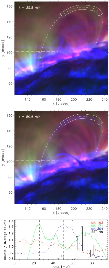
To investigate the thermal non-equilibrium scenario we have chosen a loop (hereafter loop 2, which occurs after loop 1, defined later on)in the large SDO FOV, which exhibits this gradual change of intensity from the hot to the cool AIA channels. This loop is highlighted in Figure1 in dotted lines, and it extends ≈42Mm above the surface leading to an approximate length of 132 Mm for a circular geometry. Its left footpoint is also covered by the FOV of SST. A zoom-infigure focusing on the loop is shown in Figure3, where two snapshots in the loop evolution can be seen in the upper two panels, separated by ≈24min, while the lower panel shows the integrated intensity in different AIA channels along the top part of the loop, as well as the size-weighted coronal rain intensity in Hα (defined later on) close to the loop footpoint. These panels clearlyshow a progression in the AIA channels from 193 dominated emission to 304 dominated emission. Prior to

While AIA 304 has a single-peaked light curve, AIA 193 and 171 show much more variability on the scale of a few to 10–15 min. The variations in Hα are much more extreme and on a shorter timescale than for the AIA channels, but this is to be expected considering the difference in cadence and the fact that the AIA intensities are integrated over a large area, while the Hα intensities stem from single rain clump measurements. A large quantity of Hα clumps is observed falling across the SST FOV with basically two slightly different trajectories but converging to similar locations, apparently within the umbra of the sunspot. In Figure4an example of a large clump is shown in an Hα Doppler image (±0.76Å, left panel) and in AIA filters. The track of the clump, shown in dotted lines coincides with a dark loop structure of larger width in the EUV passbands. This dark structure matches with a bright loop structure above the limb (hereafter loop 1), adjacent (to the right)to loop 2. A composite image of the SST/CRISP FOV

(Doppler image Hα±0.76 Å in red)together with AIA 171

(in green)and AIA 304(in blue)is shown in Figure5, where the same rain event as in Figure4is shown.

In order to identify all the clumps, for instance those belonging to loops 1 and 2, a semi-automatic routine was written detecting all rain-like structures crossing a specific path in the FOV (see Section 2.3). This routine calculates the intensity, Doppler velocity, the width, and the length for each clump. We select two cuts, C1 and C2, roughly transverse to loops 1 and 2, respectively, plotted in Figure5, crossed by most of the clumps. Animations 3 and 4 show the detected clumps as they cross C1 and C2, respectively(in red the FWHM of thefit to the clumps’widths). These cuts can be seen to be roughly perpendicular to the trajectory of the clumps. The algorithm confidently detects 46 and 95 clumps for C1 and C2, respectively (as shown in the animation, a myriad of smaller clumps exist, but these are too faint and cannot be confidently detected by the algorithm). Despite the apparent crossing of these loops(evidenced by the intersection of C1 and C2), these are actually well separated along the LOS (the algorithm further ensures that no clumps are common to both C1 and C2). This is evidenced by the different Doppler velocities between clumps belonging to separate loops. Indeed, clumps belonging to a specific loop will share a common trajectory and therefore a similar Doppler velocity in general. This correlation is also obtained in three-dimensional (3D) numerical simulations of thermal instability reproducing coronal rain and prominence threads (Luna et al. 2012). Figure 6 shows a histogram of Doppler velocities and derived temperatures for all detected clumps. Positive and negative values correspond, respectively, to redshifts and blueshifts. We can see that the Doppler velocities concentrate in threedifferent groups, one peaking at

30

≈ km s−1, another at≈ −10km s−1, and the last one at≈ −40

km s−1. Thefirst and second groups correspond to the clumps crossing C1 and C2 respectively, while the third corresponds to the Doppler velocities of the clumps in loop 2 at chromospheric heights (cut F2, defined in Section 4.4). The projected velocities of the clumps crossing C1 and C2 are found to be similar, with an average of 110 km s−1. This ensures that the angles of fall for each family of clumps is different, and similar within each family(as indicated by the formulae for the falling angle calculated inPaper I). We conclude therefore that the C1 and C2 clumps correspond to twodifferent loops.

The clumps crossing C2 are found to follow a dark structure in the EUV passbands similar to that plotted in Figure4. This

dark EUV structure appears bright above the limb and matches with loop 2. The geometry of the loop seen in Figure3and the direction of theflow suggest that the material is coming toward the observer, matching with the negative Doppler velocities found in Figure6for the C2 clumps. We can therefore confirm that the C2 clumps belong to loop 2.

As shown by Anzer & Heinzel(2005)the Hαintensity from filaments is strongly correlated to darkening in EUV passbands, and is due mainly to continuum absorption from neutral hydrogen, neutral helium, and singly ionized helium(and to a lesser extent to volume blocking, especially in the case of small size structures as coronal rain clumps). Therefore, both the volume and the composition of the emitting structure are

important factors that can be correlated to the detected intensity variations in the EUV passbands. In the lower panel of Figure3 we thus plot as a black histogram the Hα intensity multiplied by the width squared(assuming axi-symmetry for the clump) for the clumps crossing C2. The bulk of the distribution spans over 25 min and the peak is shifted by≈20min from the 304 peak. However, the Hα detection is made at the footpoints, while the AIA peaks arefirst observed at the apex. The clumps are observed to fall with average total speeds of 110 km s−1 and accelerations around 0.1 km s−2. Assuming no initial velocity, constant acceleration and a circular loop, the travel time of the cooling plasma is 20±10 min, which locates in time the origin of the clumps close to the 304 peak. This result supports the common origin for the Hα clumps with the rain observed in 304 in loop 2.

The temperature histogram in Figure 6 shows that all the detected clumps have very cool temperatures, mostly below 10,000 K, with a peak at 2000–5000 K. As explained in Section 2.3 these temperatures correspond to upper limits. While we postpone a discussion on these low-temperature values to the pertinent section, these results clearly indicate that loops 1 and 2 undergo full catastrophic cooling to chromo-spheric temperatures.

3.3. EUV Variation Associated with HαRain Emission

It is interesting to compare the EUV and Hα intensity variations across the C1 and C2 segments. This is shown in Figure7. For each time step we average the intensity in each channel over a small region centered around each cut. For Hα, as in Figure3, we plot the average of the intensity times the square of the width for each clump(seefigure caption for more details). Also, for the times at which a clump is detected the intensity in each EUV channel is calculated over the location of the clump only, in order to discern better a possible effect on the EUV passband for the passing clump. For the clumps crossing C1 we can see that most of the time groups of clumps close in time produce a decrease in all of the EUV intensity channels (at times t≈0, 10, 27, 40min), except 304, for which an intensity increase is generally detected. For C2 a clear correlation is also detected. Quasi-periodicfluctuations in the EUV passbands observed in the time range t = 60–90 min seem to match the Hα intensity fluctuation in the same time range. Contrary to the previous case here a maximum in the Hα intensity seems to be positively correlated with all EUV

Figure 4.Multi-panelfigure showing a snapshot of a clump falling toward the sunspot in data set 1. From left to right, a Doppler image from SST/CRISP in H 0.76

α± Å,SDO/AIA 304, 171, 193, 211, and 335. The dotted lines follow the center of the condensation, observed in emission above the spicular layer(above y≈47″)and in absorption below this layer. Notice the kink in the trajectory of the clump aty≈35″.

Figure 5.Composite image combining a Doppler image from SST/CRISP in H 0.76

α± Å(in red),SDO/AIA 171(in green)andSDO/AIA 304(in blue)for data set 1. The image shows the same snapshot of the falling clump as in Figure4, whose trajectory is indicated by the dotted curve. Four transverse cuts to the main axis of two rainy loops are shown, located at two different heights: C1 and F1 for loop 1(C2 and F2 for loop 2)at coronal and chromospheric heights, respectively. The observed clump belongs to loop 1. Animations 3–6 are zooms into thisfigure, showing the detected clumps crossing cuts C1, C2, F1, and F2, respectively(where the FWHM of thefit to the clumps’widths is plotted over in red).

passbands. Indeed, each peak of the former seems to correspond to a local peak in the latter.

3.4. Hinode/SOT, IRIS/SJI, andSDO/AIA Observations

We now turn to the second set of observations involving SOT, SJI, and AIA. A look at Figure 2 and Animation 2 immediately indicates the large presence of cool material above the active region. In red, green, and blue we show CaII H

emission from SOT, SiIV 1400 emission from IRIS/SJI, and

FeIX171 emission from AIA, respectively. We can see the

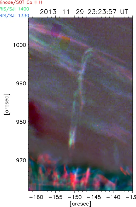
presence of two kinds of cool structures above the spicular layer. Prominence material is observed flowing relatively slowly roughly horizontally, while coronal rain is observed falling relatively faster along loops bright in AIA 171(other cool static prominence-like structures are also observed, e.g., at ( , )x y ≈ −( 160, 970)). Here we will concentrate on a loop exhibiting coronal rain, with one footpoint at ( , )≈x y ( 120, 930)− and the other apparently at( , )x y ≈ −( 150, 955), expanding in the corona up to a height of roughly40″(leading to a length of roughly 180 Mm assuming circular geometry). The rain appears from 23:12 UT to 23:30 UT(the end of the co-observation sequence)and is observed to initiate at the apex of the loop and to fall toward the farther footpoint.

A zoom-in onto the loop of interest is shown in various wavelengths in Figure8and Animation 7. Contrary to thefirst data set, here we are able to observe the chromospheric emission from the rain well above the spicular layer, but we are not able to follow it once it goes below this layer.

3.5. Cooling Through Transition Region Temperatures

In order to follow closely in time the evolution of temperature in each wavelength we plot in the upper panel of Figure9the integrated emission for eachfilter for coronal rain pixels belonging to the previously indicated loop. As seen in Animation 2, halfway through the coronal rain event a

Figure 6.Histograms of temperature(left)and Doppler velocity(right)for the Hαclumps detected with SST/CRISP in data set 1, following the method described in Section2.3. The black histogram corresponds to events whose measurements have a standard deviation above 10% of the mean. Positive and negative Doppler velocities correspond, respectively, to redshifts and blueshifts.

prominence that appears to be in the background crosses the upper portion of the loop. In order to minimally reduce such LOS projection effects, the selection of clump paths and the times and locations of rain along such paths is done manually and is done ensuring that the prominence is not along the LOS. In thefigure we can see that thefirst emission of rain appears in theIRIS/SJI images, before showing up in the CaIIHfilter. The

SJI 1400 filter comes first (att0≈44.5min), followed by a

peak in SJI 1330 (t= t0+2.5 min), then SJI 2796 (t=t0+5.5 min)and a small peak in CaIIH roughly at the

same time. The light curves generally show short-timescale variability. While all the SJI channels have a first large peak followed by gradually smaller peaks, the CaIIH emission starts

with a small peak and increases over the next fiveminutes, with the highest peak att= t0+8min. Interestingly, the time

lag between thefirst or highest peak of each diagnostic seems to increase as the rain becomes visible in each: the CII peak

follows the SiIVpeak after∼2.5 min, MgIIk follows CIIafter

∼3 min, CaIIH follows MgIIk after∼3–3.5 min. Although the

dynamic range differs, part of the increases and decreases are visible accross several diagnostics. For instance, the initial CII

peak around 46.5 min seems to coincide roughly with a secondary SiIV peak, the initial MgII k increase and peak

around 49 min is mirrored in minor by CaIIH, while AIA 304

and 171 seem to follow each other closely throughout. The behavior of the AIA filters, and especially 171, is strikingly different. Animation 2 shows that most of the loop is bright and stays bright in 171, from a first peak about 10 min before first appearance of coronal rain in SJI 1400. No EUV darkening co-spatial to the rain is observed in this case, as was the case for data set 1. Both AIA 171 and 304 increase slightly in intensity during the rain event, with the 304 emission of the rain starting att= t0+3.5min, roughly at the same time as the

MgII k emission. This is more clearly seen in Animation 7.

This behavior seems contrary to that observed in the loops in thefirst data set with CRISP and AIA, in which 171 emission at the loop apex peaks either prior or following a rain event and is at a minimum during the rain event, and in which 304 peaks after 171 and roughly at the same time or prior to Hα (cf. Figure3). Multiple small peaks are also observed in the AIA 171 emission, in a quasi-periodic fashion separated by a few

minutes, similar to the behavior observed in data set 1, shown in Figure7.

Another useful way to visualize the evolution of emission is through the cumulative light curves, plotted in the lower panel

Figure 8.Multi-panel showing a snapshot of the coronal rain event in data set 2. From left to right we haveHinode/SOT in CaIIH,IRIS/SJI 2796, 1330, 1400, and SDO/AIA 304. Each snapshot corresponds to the closest snapshot in time to that taken by SOT, and for each the average background is subtracted. The time difference of each snapshot with respect to that of SOT is indicated in the upper part of each panel.

(An animation of thisfigure is available.)

Figure 9.Light curves(top panel)and cumulative light curves(bottom panel) of the coronal rain pixels in the loop highlighted by the rain in Figure8of data set 2. In both panels theHinode,IRIS, andSDOdiagnostics are differentiated by color: CaIIH(purple), CII1330 slit-jaw(blue), SiIV1400 slit-jaw(cyan),

of Figure 9. In this figure we can see the same progression throughout the filters, with the variability reflected now in the slope of each light curve. Accordingly, the behavior between the SJI filters is very similar, characterized by two different slopes: an initial fast rise with a steep slope(untilt ≈50min) followed by a more gradual rise. The fast rise can also be seen in Animations2 and 7: the rain brightens as soon as it appears close to the apex of the loop, especially in SJI 1400 and 1330. This two-step behavior suggests two different cooling phases. The CaIIH emission appears mostly during the second cooling

phase, it has roughly the same slope throughout the evolution, reflecting a similar rise and decay of the intensity in the upper panel. Accordingly, Animations 2 and 7 show a more gradual emission in CaII H. The behavior between the AIA 304 and

171filters is very similar and constant on average, leading to a roughly constant slope in the cumulative plot of Figure9.

Figures8,9and Animation 7 further show that the emission in allfilters co-exists in the loop during most of the catastrophic cooling event, but especially during the second phase of slow cooling. This strongly suggests a multi-temperature structure for the thermally unstable loop. This is further supported by the increase of the AIA 171 intensity along the loop during the rain event. This will be further discussed in Section5.2.

The apparent mismatch with the AIA 304 channel, this one occurring 3.5 min after first occurrence in SJI 1400, could be due to the low sensitivity and lack of resolution of AIA with respect to the other instruments. A small clump will not become bright enough above the noise level unless it either increases in intensity or becomes larger. In Animation 7 we can see that AIA 304 emission is barely visible above the noise level, supporting the interpretation.

4. MORPHOLOGY

4.1. Rain Showers with Cool Cores and Associated Continuous EUV Darkenings

Figure 3 and Animation1 show that the downward flow along many of the loops in the active region seen in AIA 304 has a continuous character with little clear substructure, especially in the direction of motion. This is also observed in the lower part of the loops shown in Figure 4, where the downflow appears dark in absorption. However, as revealed by Animations 3 and 4, the falling Hα clumps observed with CRISP come in various sizes and intensities along the same paths. Figure5shows an example of a clump in Hαin emission above the spicular layer, and extending onto the disktoward the umbral region of the sunspot(marked by a dotted line in the figure). The on-diskpart of the elongated rain clump is observed as a thin absorption feature and is adjacent to other elongated rain clumps(also seen in Figure4). Surrounding the Hα emission, EUV darkening can be observed all along the clump trajectory in the lower part of the loop. This low EUV emission is more persistent, as shown in Figure 7, thus matching the continuous (as opposed to clumpy) character observed in AIA 304 in the larger FOV of Figure1. However, as shown in Figure7and described in Section3.3, a close look at this low emission reveals small EUV variations, which appear correlated to the Hα intensities. This occurs especially when several Hα clumps appear close in time. Such groups composed of a large number of small Hαclumps were denoted in Paper Ias “showers.” As predicted in that work here we show that such showers, and also a small minority of large and

dense enough Hα clumps, are associated with absorption features in EUV(and corresponding intensity variations within the dark structure). Figure 4 shows that these absorption features are significantly wider than the Hα emission(on the order of a few times the Hα width), suggesting a wide transition from cooler to hotter temperatures. Also, a comparison between Animations 1 and 3 (or 4) indicate that the EUV absorption features are significantly longer than the Hα clumps(except for the few very long clumps that extend beyond the FOV, for which we cannot confirm). These results may suggest at first a scenario in which cool chromospheric cores are surrounded by warmer diffuse shells. However, the large difference in spatial resolution between CRISP and AIA may be the main factor behind this picture.

4.2. Co-spatiality of Emission and Substructure

The previous scenario is further supported by data set 2. As shown by Figure8and Animation 7, the downflow in AIA 304 appears mostly structure-less, although with a slightly brighter head(which also appears bright in the other chromospheric and TRfilters). On the other hand, substructure can clearly be seen not only in the chromosphericfilters(CaIIH and SJI 2796)but

also in the TRfilters(SJI 1330 and SJI 1400). Close inspection further indicates a very similar rain structure suggesting a high degree of co-spatial emission in both chromospheric and TR filters. This can more clearly be seen in Figure10, which shows a composite image of CaIIH(in red), SJI 1330(in blue), and

SJI 1400 (in green). This result suggests that the lack of structure in AIA 304 may not be due mainly to a difference in temperature but rather to a lack of spatial resolution.

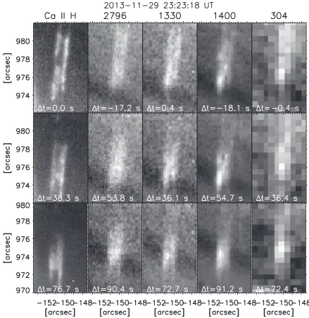
To analyze more closely the degree of co-spatiality we zoom-in into the region and follow a small shower of clumps

(the head of the rain, which appears bright in Figure8). This is shown in Figure11, where the same shower is shown at three different times along its fall, separated by ≈40s from each other. The shower’s length becomes shorter as it falls(passing from8″ to 4″). Its width on the other hand remains mostly unchanged. However, the width of the shower(and the amount of substructure)depends strongly on the wavelength. While in AIA 304 the shower appears as a single entity, the presence of substructure is obvious in CaIIH. The shower can be seen to be

composed of two strands, each one presenting inhomogeneities along their lengths. The substructure is far less evident in SJI 2796, probably due to the significant increase of opacity in this line. However, it resurfaces in SJI 1330 and SJI 1400 with similar shapes, although less clear due to the lower resolution. This picture not only proves a multi-temperature scenario for coronal rain but also proves the existence of substructure in thermally unstable loops in chromospheric to at least TR temperatures. A look at AIA 171(Animation 2)further shows that coronal temperatures are present throughout the loop, especially in the wake of the rain head.

4.3. Density for a Thick Clump

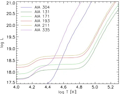
corresponding wavelengths of the absorption needs to be minimal. While these may be questionable in the present case

(a catastrophically cooling plasma could be out of ionization equilibrium if the cooling timescale is shorter than the ionization and recombination timescales; also, as shown previously, we have a strong degree of density inhomogeneity within the rain) the results of the applied technique can nonetheless provide important density constraints and clues on the state of the plasma. Here we do this for a large clump producing enhanced EUV darkening, similar to that shown in Figures 4 and 5, but we postpone a full investigation on densities to future work. In Figure 12we plot theL function, defined in (Landi & Reale 2013, formula 9), which, at temperature of absorption is equal to the hydrogen column density. Our case is similar to their special case 2(Section 3.2 in their paper). The background emission is measured at the same locations where the EUV darkenings are observed but at times where no Hαclumps are observed(we take a few time steps prior and after the passage of the clump, and then take the average of the two). The EUV intensities are taken over the trajectory of the clump, seen as darkened streaks in an x− t

plot. In the calculation of L we further assume a helium abundance of 5%. In Figure 12we can see that the region of

intersection of all curves is concentrated inlogTabs=4.4 4.6−

andlogL =18.1 18.7− cm−2(whereTabsis the temperature of

maximum absorption). Assuming axi-symmetry along the direction of propagation, the LOS depth across the clump is then roughly equal to the clump’s width. The clump’s width in the EUVfilters is 2. 8″ , although it cannot be determined with precision due to the poor spatial resolution of AIA. The clump in Hαhas a maximum width of0. 6″ (with an average of0. 4″ ). From the results of data set 2, it is likely that the larger widths in EUV are mostly an effect of the lack of resolution(which would smear out the width a factor proportional to AIA’s PSF). We therefore assume an EUV width 1.5–2 times larger than the Hαwidth, leading to a width of roughly 700 km. This leads to an electron density of 1.8–7.1 × 1010cm−3, where the scatter is most likely due to the presence of inhomogeneities within the clump. This is supported by the fact that the spectral width of the clump in Hα indicates a temperature of 5500±500 K, suggesting a multi-temperature structure, and possibly a higher density. Assuming a constant pressure within the clump the core density can then be up to2.5_×1011_cm−3_.

4.4. Clumpy Versus Continuous

As the clumps fall further down toward the sunspot in data set 1 they become absorption features in the wing of Hαwhile they gradually become bright toward line center(see Figures4 and5). These distinctive features allowus to trace them down to chromospheric levels, just before impact. Similarly as previously done for coronal heights we define two cuts at chromospheric heights roughly perpendicular to the clumps trajectories, F1 and F2, corresponding to loops 1 and 2, respectively. Both C and F pairs are plotted in dashed curves in Figure 5. As in Animations 3 and 4 for C1 and C2, Animations5 and 6 show the detection of rain clumps across F1 and F2, respectively (in red the FWHM of the fit to the clump’s width). These animations indicate that the C1 clumps fall either into the umbra or toward the closer edge of the sunspot (projection effects do not allow us tofirmly pinpoint the location of the fall)and the C2 clumps seem to fall mainly toward the far edge of the sunspot. Tracing of coronal rain clumps to such low heights has never been achieved before and is possible here thanks to the high falling speeds of the clumps

(which produces the dark absorption features in the wing of Hα)and to the high spatial and temporal resolution of CRISP. Indeed, the total velocities(taking into account projected and Doppler velocities)vary between 80 and 120 km s−1for both loops.

Due to the increase of projection effects at low heights, the high speed of the clumps and the seeing effects(which do not alway provide clear subsequent images), it is not possible in most cases to specify the start and end for a clump at low heights, and therefore provide a robust determination of clump lengths. It is therefore possible that two subsequent detections at the same location correspond to the same clump. Also, it is highly likely that many of the clumps detected at heights C are detected again at heights F. However, since we are more interested in regarding the rain as aflow rather than a discrete set of condensations(especially because their morphology can change dramatically as they fall), for our statistical analysis we consider that all clumps are different (and for the lengths we give an approximate value determined visually). Since there are many clumps that fail to be detected by the algorithm(due to

the previously stated reasons), we consider that this procedure leads to a better approximation to the real rain population.

A striking feature shown by Animations 5 and 6 is that at such low chromospheric heights the clumps appear signifi -cantly less clumpy (their lengths increase)and the downward flow becomes continuous and rather persistent. In order to quantify this effect better we plot in Figure 13a histogram of clump detection weighted with their respective widths squared at the two previously defined heights for loops 1 and 2. Not only are the clumps in the corona detected at later times in the chromosphere, but we also detect many more rain crossings at those lower heights, indicating an increase in the rainflow with decreasing height (46 and 145 clumps for C1 and F1, respectively; 95 and 193 clumps for C2 and F2, respectively). In Section5.4we discuss possible reasons for this increase in clump occurrence at low chromospheric heights.

4.5. Strand-like Structure

As shown in Section 4.2, the presence of substructure in coronal rain at high resolution is not only clear at chromo-spheric temperatures such as those of CaIIH and SJI 2796 but

also at higher temperatures, such as those of SJI 1330 and SJI 1400. As shown in Figure11, as the rain falls substructure is observed to be organized along strands of various lengths but rather similar widths. This is also observed in Animation 7 for the rest of the rain in this event and in data set 1 at even higher resolution. Indeed, at the highest resolution achieved in this work(in Hαwith CRISP)similar strand-like structure appears, as shown in Figure 4 and Animations 3–6. Due to the very dynamical nature of coronal rain it is not easy to discern the strand-like structure traced in time by the rain. For this, we plot in Figure 14 the time variance in a Doppler image in Hα± 0.6Å over a time period of 22 min for loop 1 and its

Figure 11.Substructure for a rain shower in the rain event of data set 2. The shower corresponds to the head of the rain and is shown at three different times separated by roughly 38 s from each other(shown in the rows)and for different wavelengths(shown in the columns). From left to right we haveHinode/SOT in CaIIH,IRIS/

surroundings(where the time variance is defined as the sum of the squared average-subtracted intensity for each pixel). Thanks to the emission features of the rain in the wing of Hαboth above the spicular layer and at chromospheric levels, the clumps produce bright traces in the variance image. These traces appear as various strands at both of these heights(in the

figure, these are visible from50″to55″ and28″to35″in the vertical axis). In the figure, 6–8 strands with widths around

0. 2 0. 4″ − ″ can be discerned at both heights, although a larger number may exist due to projection effects. It is worth noting that the 22 minuteperiod over which the variance is taken is a significantly long time for coronal rain. Indeed, the number of clumps detected over this time period is on the order of 60–70. Also, as calculated previously in Section3.2, the travel time for rain in these loops is on the order of 20±10 min. Last, numerical simulations indicate that the catastrophic cooling part of limit cycles is generally short, under an hour or so

(Mendoza-Briceño et al. 2005; Antolin et al. 2010; Susino et al.2010; although this depends on various parameters of the heating). Therefore a significant part of the catastrophic cooling for this loop may be captured in the time variance, strongly suggesting that the clumps follow well-defined fundamental magnetic structures in the corona.

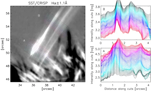
Interestingly, apart from the prominent clumps as those in Figure 11, the surrounding diffuse atmosphere in data set 1, dimly bright in Hα,also appears structured in the same way. This is especially clear at times of large clumps. An example of this is shown in Figure15, where a snapshot of a falling clump can be seen in Hα±1.1Å. A bright clump with a long tail can be seen and, particularly, multiple strand-like structures next to it, as ripples with similar widths down to0. 15″ or so, uniformly distributed within4″ of the clump. This structure can still be

Figure 12. Lfunction (in logarithmic scale), as defined in Landi & Reale (2013), with respect to temperature, for the various AIAfilters calculated over the trajectory of a rain condensation producing EUV darkening.

Figure 13.Histograms of rain condensations detected in Hαwith SST/CRISP for data set 1 along cuts C1, F1 and C2, F2 for loops 1 and 2, respectively. The condensations detected at coronal heights(C cuts)constitute the deep blue histogram, while those detected at chromospheric heights(F cuts)constitute the light blue histogram. The histograms are constructed by taking a bin size of a 100 s, and for each time bin the intensity of all contained clumps are summed, each multiplied by the clump’s width squared.

discerned (although with decreasing intensity) when shifting the wavelength position over a range of±0.5Å around1.1Å, ruling out possible instrumental effects from the narrowband CRISP wavelength channels. In order to show the strand structure better we make transverse cuts across the clump at two different locations, one at the head and one at the tail of the clump. The Hαintensity along these cuts is shown in the right panels of thefigure. Next to the large peak corresponding to the bright clump, around 8 ripples can be distinguished extending significantly along the direction of propagation. This structure is highly reminiscent of the MHD thermal mode (also known as the entropy mode in the absence of thermal conduction),first predicted by Field (1965) and later developed by van der Linden & Goossens (1991a, 1991b), Goedbloed & Poedts

(2004), Murawski et al.(2011). Indeed, the spatial distribution of such mode is that of a main elongated dense clump with multiple smaller clumps side by side of similar widths. The generation of this wave is guaranteed by the small but non-zero perpendicular thermal conduction in the corona. Although static in an ideal scenario, this wave is expected to move together with theflow. In this scenario, the observed strand-like structure at the smallest detected scales could be the result of MHD thermal modes produced from thermal instability.

4.6. Sizes

We now turn to the statistical determination of sizes. The methods used in the widths and lengths calculations are explained in Section 2.3. The routines used for this detection are semi-automatic. The detection of a clump is rather strict,

and is based on several conditions which rule out most of the fainter and smaller clumps at diffraction limit resolution. For instance, the smaller widths that can be discerned in the cross profiles in Figure 15 are mostly left out by the algorithm, in favor of precision and reduction of errors.

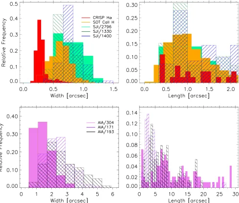
In Figure 16 histograms displaying the relative frequency

(for each wavelength)for the obtained widths and lengths are shown, combining data sets 1 and 2, and therefore all the instruments used in this study(note that the bin widths of the distributions have been set equal to the resolution of each instrument). Due to the large number we restrict the histograms to the more interesting small scales part (upper panels) and separate between the high (CRISP, SOT, SJI) and low resolution instruments (AIA in the lower panels). The figure clearly shows a significant difference between widths and lengths at all wavelengths. The widths appear nicely dis-tributed, with increasingly higher occurrence frequency at smaller scales for each wavelength and a tail at longer scales. Such distribution shape seems therefore independent of temperature, with an apparent peak for all clumps between

0. 2″ and 1. 1″ . Hα and CaII H clump distributions have,

respectively, narrow and broad peaks at0. 25″ and0. 6″ . Blobs observed with IRISin SJI 2796, SJI 1330 and SJI 1400 have similar distributions peaking at0. 6″ − ″0. 8. We note, however, that SJI 2796 presents a broader distribution for the peak, between 0. 6″ and 1″, probably due to the higher opacity compared to the optically thinner CIIand SiIVlines. For AIA

we note that while widths in 171 and 193 peak around1. 8 3″ − ″, 304 peaks around0. 8″ − ″1. 7.

On the other hand, the lengths show a more random distribution, although with high clustering at small numbers, between 0. 5″ and 1. 5″ . It is worth noting that the lengths distribution spans up to30″or so(for instance, the very long clump of Figure 4). For lengths longer than 5″ (not shown here)the distribution becomes sparse.

In Table1 average values for each wavelength and data set are shown, together with the total number of clumps detected in the FOV per minute as an indication for the number of clumps detected in each data set. We choose to calculate this number since a clump is a not well-defined plasma structure over time. As shown in the present animations(and in Figure11)and in Paper I, clumps can dramatically change shape, appear and disappear along their fall. This number needs to be read with caution: the area over which rain is detected in data set 1 is roughly half that in data set 2 (therefore, dividing the number over area would lead to a similar number between SST and Hinode). The continuousflow in 304(as opposed to clumpy)

also makes it difficult to identify a clump. For AIA only clear cut examples of clumps were selected, which explains the low number per minute.

The widths presented here in Hα are similar to previously measured widths in the same wavelength with CRISP in large statistical data sets (Antolin & Rouppe van der Voort 2012; Antolin et al.2012), but present a relatively higher number of clumps at lower spatial scales. This is mainly due to the fact that the CRISP instrument gained from improved spatial sampling after an upgrade performed in 2009. The widths of CaII H clumps are similar to those reported in Antolin et al. (2010). In the top left panel of Figure 16 the tendency of number increase for clumps with smaller widths suggests a tip-of-the-iceberg scenario.

As expressed previously, the lengths appear to be more randomly distributed, especially in Hα, and therefore may be more data set dependent. For instance, extremely long clumps are only observed in data set 1, and have not been previously

observed in other data sets in Hα with CRISP, except in the recent work by Scullion et al. (2014)in the context offlares, i.e., stronger footpoint heating sources.

5. DISCUSSION

5.1. EUV Intensity Variations as a Signature of Catastrophic Cooling

Coronal loops in active regions often present intensity variations, which are regularly associated with states out of hydrostatic equilibrium such as states of thermal non-equilibrium (Aschwanden et al. 2001; Reale 2010). A state of thermal non-equilibrium implies the presence of thermal instability in coronal loops. This instability can be thought as the most general state of the plasma (meaning that thermal equilibrium is extremely unlikely). The relevant question here is what are the timescales of this instability in coronal loops? Accordingly, this instability can have a complete character, in the sense that runaway cooling due to the shape of the optically thin loss function may occur locally in coronal loops and continue uninterrupted down to chromospheric temperatures, until heating from local sources overcome the losses due to its own radiation. The completeness of thermal instability, however, is not guaranteed and depends strongly on the efficiency of the heating mechanisms and on thermal conduc-tion. Mikić et al. (2013) have shown that even changes in geometry(non-uniformity in area cross-section and asymmetry in the heating)play an important role in determining the aspect of this instability. Furthermore, the spatial scales involved in the cooling processes(for instance, the clumpiness and strand-like structure of the rain)are directly related to the properties of the plasma and to the counter-acting heating mechanisms, and may therefore reveal essential characteristics of the heating processes.

Despite the close link between thermal instability and coronal heating and therefore the importance of thermal instability, we do not know how ubiquitous this instability is in the corona and the details of its character (for instance, whether it is complete or not). This is largely due to the high complexity of the thermal instability in strongly anisotropic plasmas such as the solar corona. Recent observational studies over active regions indicate a general tendency for cooling

(Viall & Klimchuk2012). Although it is clear that not all the loops in an active region are in a thermal non-equilibrium state and undergo catastrophic cooling, it is important to estimate what fraction of loops are.

The traditional picture of thermal instability implies that coronal loops in a thermal non-equilibrium state become progressively cooler, suggesting a time delay between filters detecting emission at different temperatures. Such cooling progression throughout TR temperatures has previously been invoked to explain variations in EUV light curves ( Fou-kal 1976, 1978; Kjeldseth-Moe & Brekke 1998; Schrijver 2001; O’Shea et al. 2007; Warren et al. 2007; Landi et al. 2009; Tripathi et al. 2009; Ugarte-Urra et al. 2009, 2006; Kamio et al.2011). However, the direct link to catastrophic cooling has not been yet firmly established, since all of these multi-wavelength observations do not include chromo-spheric ranges. In this work we make the first steps in this direction by linking commonly found intensity variations in EUV filters of SDO/AIA to the observational imprint of catastrophic cooling, i.e., coronal rain observed in chromo-spheric diagnostics.

We observe complete thermal instability with temperatures down to the chromospheric range. In Section 3 we show that EUV darkening is found to be associated withflows in AIA 304 and presents a continuous and rather persistent character. Such AIA 304 flows are observed along many of the loops within the active region(data set 1), part of which are captured toward the footpoints in Hαby CRISP. The flows in AIA 304 appear strongly correlated in space to the appearance of cool chromospheric material in the loops observed in Hα, which occurs in a more intermittent way. This suggests that while the entire loop may be thermally unstable and cooling, plasmas at TR temperatures are more widespread and common within the loop than plasmas at chromospheric temperatures. This is expected to some extent due to the tendency of the plasma to keep a uniform pressure distribution along the field (and the fact that thermal instability entails a local loss of pressure leading to small condensations).

Small EUV intensity perturbations are further strongly correlated in time with the presence of Hα rain clumps. Although intermittent, these clumps can come in series of events and generate quasi-periodic EUV intensity variations on the order of a few minutes. In most cases, these variations are found to be associated with groups of chromospheric clumps which we have previously termed “showers” (Paper I), and span over a few arcseconds in the transverse direction. Correlation between EUV darkening and Hα has been extensively studied in the case of prominences (Heinzel & Anzer2006; Labrosse et al.2010). For the EUV wavelengths of interest here, this correlation is mainly due to continuum absorption from neutral hydrogen, neutral helium, and singly ionized helium.

Table 1

Average Values for Both Data Sets

Instrument Data Set Width Length Blobs

and Filter (arcseconds) (arcseconds) (/minutes)

CRISP Hα 1 0.3±0.093 3.85±5.77 5.

SOT CaIIH 2 0.61±0.17 1.05±0.51 9.7

SJI 2796 2 0.8±0.19 2.49±1.97 2.6

SJI 1330 2 0.7±0.15 1.75±1.35 3.7

SJI 1400 2 0.8±0.17 1.76±1.26 4.6

AIA 304 2 1.56±0.15 10.8±6.5 2.2

AIA 304 1 1.4±0.7 12.7±9.2 1.2

AIA 171 1 2.45±0.81 5.5±5.2 1.2

AIA 193 1 2.69±1.07 7.4±4.6 1.2

Note.Averages are calculated over all detected blobs in both data sets. Row order is set according to increasing temperature. For data set 1 the measurements are limited only to the rain detected in loops 1 and 2. For data set 2 the measurements are limited to the loop shown in Figure8. While each measurement is itself an average value over a large quantity (see Section 2.3) and therefore has its own standard deviation, the standard deviation shown here for widths(lengths)is simply taken over the set of blob widths(lengths). The last column provides the number of blobs detected per minute for each data set, which implies dependence over the FOV over which this detection is carried. For the SST, the detection is done over a small part of its FOV(roughly 5″× 17″), which is much smaller than the FOV for theSDO

5.2. Multithermal Character

The progressive cooling picture from thermal instability also suggests a difference in emission with height. In this picture, emission in Hα and at cooler wavelengths is preferentially detected at low coronal heights. In the middle panel of Figure17we plot the averages of height versus temperature for all detected clumps in data sets 1 and 2. The temperatures taken for the SJI and SOTfilters are those of maximum formation for the dominant ions of eachfilter. Those for CRISP correspond to the measured temperatures, shown in Figure 6. Although not strongly correlated, the plot suggests a slight temperature decrease with height. Particularly, the very low temperatures below 5000 K, even down to 2000 K or so, for the Hαclumps detected with CRISP at the lower part of the loops provides support to the cooling picture.

Through co-observation between IRIS and Hinode/SOT we are able to follow for thefirst time the rapid progression in the runaway cooling in thermally unstable loops. A two-step progression is found in which fast sudden appearance at TR and upper chromospheric temperatures is followed by a more

gradual appearance at lower chromospheric temperatures. This two-step scenario agrees with the shape of the optically thin loss function, which predicts runaway cooling down to 105K or so, below which material becomes progressively optically thick, and therefore radiation has a lower escape probability

(leading to less efficient radiative cooling).

Despite the progressive cooling from transition temperatures to chromospheric temperatures found in data set 2 the AIA 171 intensity along the loop is found to increase about 10 min prior to the rain event, and remains bright and even further increases at the end, during the rain event. Such behavior strongly suggests the presence of multithermal plasma in the loop, from chromospheric to coronal temperatures. Further-more, it implies that the progressive cooling picture down from coronal temperatures to chromospheric temperatures is not always reflected in the evolution of EUV light curves. Hot material can co-exist with catastrophically cooling plasma. Therefore a hot to cool systematic sequence in EUV channels is not an observable requirement for a loop in a thermal non-equilibrium state.

The obtained cooling down to chromospheric temperatures is very fast, achieved in a timescale that varies from tens of minutes(data set 1)down to minutes(data set 2). Due partly to this reason, in both analyzed data sets, and especially in the one analyzed with SJI and SOT, thanks to the high spatial and temporal resolution, we find a high degree of co-spatiality in the multi-wavelength emission over the entire span of the event. This strongly supports the presence of multithermal plasma in these loops. Furthermore, the multithermal character is accompanied by strong density inhomogeneity, which suggests a complex thermodynamic evolution within the same loop. The multithermal picture is also supported by the results of Scullion et al.(2014), which show Hαemission with CRISP co-located with EUV AIA 171 in post-flare loops.

The large range of temperatures we detect imply that coronal rain, as a result of catastrophic cooling, is not solely a chromospheric phenomenon but a TR phenomenon as well. Actually, since it is material cooling from coronal temperatures and, as discussed previously, it is more pervasive in TR temperatures, it is mainly a TR phenomenon which spans down to chromospheric temperatures if the thermal instability is complete. This result matches well the picture that is being perceived with increasing frequency in SJI and AIA synoptic observations, namely, that basically every active region shows rain-like phenomena in AIA 304 and SJI 1400. A proper statistical analysis of this picture is left as future work.

For data set 1, the EUV emission(darkening or brightening) in AIA 304 is found to be wider than the chromospheric emission in Hα or CaII H suggesting a wide transition from

chromospheric to TR temperatures. However, the highly co-spatial emission obtained from SJI and SOT in data set 2 suggests that the wide transition in data set 1 is mainly due to the lack of resolution in AIA. The observed thin transition in data set 2 must exist on spatial scales below the resolution of IRIS, i.e., 0. 33″ , which is also supported by the similar width distributions obtained with SOT and the SJI filters (see Figure16). Indeed, when closely comparing the substructure of clumps, small structural differences appear between the clumps in CaII H and in SJI 2796, 1330, and 1400. This

multithermal plasma picture and the large-density inhomogene-ities at such high resolution suggests that the thermal instability mechanism in a strongly anisotropic magneticfield such as the

Figure 17. Diagrams showing relationship between various quantities. As quantities we have the height of the measurements, estimated from the footpoint location of the loop in the chromosphere, the width of the condensations and the temperature of the condensations. For each quantity