Principles of Quantum Mechanics and Laws of Wave Optics from One Mathematical Formula

(1)

ISSN Online: 2152-7393 ISSN Print: 2152-7385

DOI: 10.4236/am.2019.1011064 Nov. 11, 2019 892 Applied Mathematics

Principles of Quantum Mechanics and Laws of

Wave Optics from One Mathematical Formula

Do Tan Si

Ho Chi Minh City Physical Association, Ho Chi Minh City, Vietnam

Abstract

Finding that in the formula of expansion of a function f

( )

r into a series of wave-like functions exp

( )

ikr the coefficients are its Fourier transforms, if existed, we deduce mathematically all the principles and hypothesis that illus-trated physicists utilized to build quantum mechanics a century ago, begin-ning with the duality particle-wave principle of Planck and including the Schrödinger equations. By the way, we find a simple Fourier transform rela-tion between Dirac momentum and posirela-tion bras and a useful permutarela-tion relation between operators in phase and Hilbert spaces. Moreover, from the found particle-wave duality formula we prove and obtain again essentially by mathematical analysis all the laws of wave optics concerning reflections, re-fractions, polarizations, diffractions by one or many identical 3D objects with various forms and dimensions.

Keywords

Fourier Transform in Quantum Mechanics, Permutation Relations between Operators, Laws of Wave Optics, Diffractions by Multiform Identical Objects

1. Introduction

From the find that a function f

( )

r may be expanded into a series of functions

eikr_{with coefficients equal to}

( )

₂_π 3 2_{multiplies the Fourier transform} _f

( )

_k

of f

( )

r we arrive to obtain that a particle moving with celerity v0,

momen-tum p0 creates a wave, confirming the wave-particle duality principle

con-ceived by Planck and Einstein in 1900-1905. Moreover we obtain that p0 is

in-versely proportional to the wavelength of this wave conformed with the hypo-thesis of de Broglie and that the particle’s energy is proportional to the wave’s frequency conformed with the proposition of Planck. The coefficient of

propor-How to cite this paper: Si, D.T. (2019) Principles of Quantum Mechanics and Laws of Wave Optics from One Mathe-matical Formula. Applied Mathematics, 10, 892-906.

https://doi.org/10.4236/am.2019.1011064

Received: October 11, 2019 Accepted: November 8, 2019 Published: November 11, 2019

(2)

DOI: 10.4236/am.2019.1011064 893 Applied Mathematics

tionality is then identifiable with the Planck’s constant h.

The Exclusion principle of Pauli may be explained by the assimilation of two particles having the same momentum and the same position with only one hav-ing double momentum so that the de Broglie wavelength is divided by two which is a paradox.

From the fact that δ

(

p p− 0

)

represents the momentum-representation of

the state p0 and

( )

1 0

3 2 2 − ei −

π p r_{its position-representation we obtain the}

re-lation k =FT r where

p

=

k

_{. These relations lead to the canonical} com-mutation relations r pˆ ˆj, l =i

δ

jlIˆ, E i= ∂ t of Born which in turn lead to

the well known Schrӧdinger equations. Utilizing the relation k =FT r we see also that the Heisenberg’s incertitude relation ∆ ∆ >x p 2_{is a matter of}

Fourier transform relation between the rectangular function

(

)

(

)

(

)

1

a H k a H k a− ₊ ₋ ₋ _{and the function} _sin

_{( ) ( )}

ax ax , H x

( )

being the Heaviside function.

Consider an atom having a discrete spectrum of states each having a value of energy Ej. It is represented by

(

)

1

N

j j

E α δ E E

=

∑

− _{. By searching the}

max-imum values of t α 2_{we see that from time to time there have emission/ab-}

sorption of a wave having frequency 1

(

)

jk h E Ek j

ν

₌ − ₋

conformed with the theory of Bohr. Besides we obtain permutation relations between functions of creation and annihilation operators in second quantization.

By the same formula giving quantum mechanics’ principles we realize that the product of a wave eik r0 and an object described by a function f

( )

r is a sum

over eikr_{with coefficients equal to}

( )

3 2

(

)

0

2π f k k− . This opens a simple way to calculate the amplitude of diffraction of a wave by a 3D object such as a semi-space which leads to the Descartes, Snell’s laws, Fresnel equations, then by a set of identical objects having different geometric forms such as plane which leads to the Braag’s formula, pyramid, sphere, etc.

Details of the finds are explained successively in the following paragraphs.

2. Obtaining Principles and Hypothesis of Quantum

Mechanics

2.1. The Wave-Particle Duality Principle

Let us expand a function f

( )

r having Fourier transform on a basis of expo-nential functions

( )

ei k

f _r =

∑

c _k kr

(2.1.1)

where k belongs to an infinite set of vectors obeying the condition that the scalar product kr is dimensionless for the following relation to hold

( 2 )

ei 1 ei ei + π

= ⋅ = kr

kr kr _(2.1.2)

(3)

( )

( ) (

)

( )

0 0 3 3 3 0 3 0

e d e e d

2

i i i

k R R k f c c c δ − ₌ −

= π −

= π

∑

∫

∑

k r _{r r} _k k r kr _r

k k k

k

(2.1.3)

so that we may state the theorem:

“Any function f

( )

r having Fourier transform may be written under the form

( ) ( )

3 2

( )

2 ei

f = π

∑

f kr

k

r k (2.1.4)

where kr isdimensionlessand f

( )

k istheFouriertransformof f

( )

r

( )

( ) ( )

( )

3 3 2

2 e i d

R

f ₌FTf _{= π} − − f

∫

kr

k r r r

_(2.1.5)

Now from the well known formulas

(

)

eax

( )

f x a₊ ₌ ∂ f x

(2.1.6)

( )

x

FTD f x =FTf x′ =ikFTf x _(2.1.7)

we get

(

)

( )

1 2

e aDx e iak eiak 2

FT x a

δ

₋ ₌FT −

δ

x ₌ − FT x

δ

₌ − _π − _(2.1.8)

so that by (2.1.4)

(

)

0 ( 0)

0 ei ei ei

k k

δ

_{r r}₋ ₌

∑

−k r kr ₌

∑

k r r −

(2.1.9)

Consider a particle situated at the position r0 and having a mass m and a

constant celerity v0. Defining

0 0

0 0 0

2 2

λ ν λ π π = =

v

k n (2.1.10)

where λ0 has the dimension of a length as it must be for k r0 to be

dimen-sionless we see from (2.1.9) that the formula

(

)

(

)

0( 0)

₍

₎

0 0 0

0 2

ei exp_i

δ

λ

−  π 

− − = =  − 

 

k r r

k k r r r r n (2.1.11)

represents at the same time this particle and a wave. Thank to the property

2

e± πi ₌1_{this wave has a wavelength} 0

λ and consequently a period

0 0 0

T =λ v _(2.1.12)

The wave function of this particle is then within a multiplicative constant

( )

(

)

0 0 0

0 2

, exp

r t A i t

T

 π  Ψ = _ − − _

k r r 

(2.1.13)

(4)

2.2. The de Broglie Particle-Wave Hypothesis and the

Planck-Einstein Relation

As

// // =m

k v p v (2.2.1) we may define a universal constant

θ

having dimension _{ML T}2 −1_{then link}

p

_with _k_{by the relation}

2 2

θ θ θ λ ν λ

π π = = =

v

p k n (2.2.2)

in order to get the form of the relation between momentum and associated wa-velength

2

p θk θ

λ π

= = _(2.2.3)

in accordance with the hypothesis proposed in 1923 by de Broglie [3].

The wave function of the considered particle may then be put under the form

( )

1

(

)

0 0 0

0 2

,t Aexpi t

T

θ

−  π 

Ψ = _ − − _

 

r p r r (2.2.4)

By dimensional consideration we see that the quantity

0 2

T

θ π

is an energy that we baptize E0 and propose to assimilate it with the energy of the quoted

par-ticle

0 0 2

E T

θ π

= _(2.2.5)

By comparison with the formulae of Planck-Einstein [1] [2] and de Broglie [3]

h E

T

= _, p h

λ

= (2.2.6)

we get the identifications

2

h

θ

= =

π (2.2.7)

=

p k

_(2.2.8)

and see that k is the commonly called wave-vector of a wave.

From now all we say that k and

r

are Fourier transform reciprocal as so as 2 1_E

T

−

π₌

and the time t. The Planck constant h was measured by Millikan

[4] in 1916. The best current value for h is _{6.62607004 10 m kg sec}_× −34 2_⋅ _{and is}

officially utilized from the date 20-05-2019 on to define the value of the kilo-gram.

2.3. The Pauli Exclusion Principle

(5)

posi-DOI: 10.4236/am.2019.1011064 896 Applied Mathematics

tion they may be assimilated to one particle with momentum 2p so that the dual wave must have its wavelength divided by 2. This leads to a paradox and confirms the Exclusion principle of Pauli [5]. For photons with momentum

p h c= ν _{too small, two times of it is quasi equal to it so that there is no}

para-dox, i.e. many photons may occupy one position.

2.4. Obtaining the Fourier Transform Relation between Bras

k

and

r

In a Hilbert space of Dirac kets and bras let according to (2.1.13)

( )

3 2

( )

0 2 exp i 0

− = π

r k k r (2.4.1) be the position-representation of a state having a definite wave-vector k0

. From the formula

( )

( 0)

( )

(

)

0

3

3 2 3 2

0

ei 2 e i d 2

R

FT − − −

δ

= π

_∫

k k r = π −

k r _r _{k k} _(2.4.2)

and (2.4.1) we have

( )

3 2 0

(

)

0 2 ei 0 0

FT FT − δ

= π k r = − =

r k k k k k (2.4.3)

so that, because k0

is arbitrary, we get the interesting relation

FT =

k r (2.4.4) which gives precision to the latent idea in many researchers that there exists somehow a Fourier relation between momentum and position:

“Inquantummechanicsthewave-vectorbra k istheFouriertransformof thepositionbra r ”.

From (2.4.4) we get the relation between momentum-representation and posi-tion-representation of a state

FT

Ψ = Ψ

k r (2.4.5)

2.5. The Canonical Commutation Postulated by Born

In the Hilbert space of states besides Xˆ and Pˆx let us formally define another

operator Dˆx

by the relation

ˆ ˆ_x ˆ ˆ_x ˆ

D X XD− ≡I_(2.5.1)

where Iˆ is the identity operator.

Now, in the space of functions let X be the operator of multiplication by x

and Dx

the derivative operator

( )

Xf x =xf x _; D f x_x

( )

= f x′

( )

_(2.5.2)

verifying

,

x x x

D X D X XD I

  ≡ − ≡

(6)

We must be attentive on the fact that the operators X D P D , , ,_x _x _p act on func-tions and X D P Dˆ ˆ ˆ ˆ, , ,x x p_x act on bras and kets.

From (2.5.1), (2.5.3) we get

(

)

(

)

'0 '0 0 '0

ˆ ˆ_x ˆ ˆ_x ˆ_x

x D X XD x− = x −x x D x =

δ

x x− _(2.5.4)

(

0

)

(

'0

)

0 x

D X x −

δ

x x− = (2.5.5)

(

D X XDx − x

)

δ

(

x x− '0

) (

= x x D0−

)

x

δ

(

x x− '0

)

=

δ

(

x x− '0

)

(2.5.6) so that

0 0

ˆ_x _x

x D x =D x x _(2.5.7)

Besides we have also

(

)

0 0 0

ˆ

x X x =x x x

δ

− = X x x _(2.5.8)

so that, as x0 is arbitrary,

ˆ_x _x

x D ≡D x _; x X X xˆ ≡ _(2.5.9)

The above relations associated with (2.4.4) and

( ) ( )

₂ 1 2 _eikx

( )

_d

( )

k k

FTxf x − ∞ i − f x x i F x

−∞

= π

_∫

∂ = ∂ _(2.5.9)

lead to

0 0 0

ˆ ˆ

ˆ

k k k

k X k FT x X k FTx x k

i FT x k i k k k iD k

= =

= ∂ = ∂ = (2.5.10)

i.e.

ˆ ˆ_k ˆ_p

X iD≡ ≡i D (2.5.11) Similarly by repeating the reasoning with P Dˆ ˆx, p_x we get

ˆ ˆ

x x

P = −i D (2.5.12) Extension to 3D space gives

ˆ ˆ

ˆ≡ ∇ ≡ ∇i _k i _p

r (2.5.13) and finally the commutation relations

ˆ ˆ

ˆ ˆj, l ˆj, l jl

r p i r  i δ I

  = − ∇ =

    (2.5.14)

which have been called quantum conditions and postulated by Born in 1925 [6]. Similarly from the fact that 2 1_E

T

−

π

= and t are Fourier reciprocal we have

t

E i= ∂ _(2.5.15)

2.6. The Schrödinger Equations

From the relations (2.5.6) we may also get an important proposition: “Theeigenvalueequation

( )

ˆ ˆ_,

(7)

of an arbitraryoperator A X P

( )

ˆ ˆ, leadstothedifferentialequationforthe func-tion xα

( )

ˆ ˆ_,

(

_,

)

x

x A X P α =A X i D x − α =a xα (2.6.1) For example, with

( )

ˆ ˆ_, 1 ˆ2

( )

ˆ

2

A X P P V X

m

≡ + (2.6.2)

we obtain the well known time independent Schrödinger equation [7]

( ) ( )

( )

2 2

2_m D V xx x E x

− ₊ _Ψ _{= Ψ}

 

 

(2.6.3)

As 2 1_E

T

−

π₌

and t are Fourier transform reciprocal we get the time depen-dent Schrödinger equation

( )

2 2

2 , , ,

2m x V x t x t i t x t

₋ ∂ ₊  _{Ψ = ∂} _Ψ  _∂ 

 

_(2.6.4)

2.7. The Heisenberg Uncertainty Principle

Let S k k

(

,∆

)

be the function equal to zero for k > ∆k 2 and to

( )

∆k −1_for

2

k < ∆k as illustrated by Figure 1.

A state α where there is incertitude on the wave-number k

(

k0− ∆k 2

)

≤ ≤k

(

k0+ ∆k 2

)

(2.7.1)

corresponds to the momentum-representation

(

)

0

(

)

0, e k k ,

k

α

₌S k k₋ _{∆ =}k − ∂ S k k_∆

(2.7.2) Utilizing the Heaviside function we may write

(

,

)

H k

(

k 2

)

H k

(

k 2

)

S k k

k

+ ∆ − − ∆ ∆ ≡

∆ (2.7.3)

Thank to (2.1.6), (2.1.7) and the property

(

)

( )

1

( )

2

2 2

2

2 e e

1

e 2

k

k _{k ix}

k ix

FTH k k FT H k FTH k

x

ix δ

∆ _∂ ∆

∆ −

+ ∆ = =

  = π _ + π _  

(2.7.4)

[image:7.595.140.540.67.737.2]

we get by Fourier transform of (2.7.3)

(8)

(

,

) ( )

2 12sin

₍

(

₎

2

)

2

x k FTS k k

x k − ∆ ∆ = π

∆ (2.7.5)

so that by (2.7.2)

(

) ( )

₍

(

₎

)

0 1₂ 0 sin 2

e , 2 e

2

k

k ik x x k

FTFT x FT k FT S k k

x k

α ₌ α ₌ − ∂ _{∆ = π} − − ∆

∆ (2.7.6)

( )

2 1 2e 0 sin

₍

(

₎

2

)

2

ik x x k

x FTFT x

x k

α α − ∆

= − = π

∆ (2.7.7)

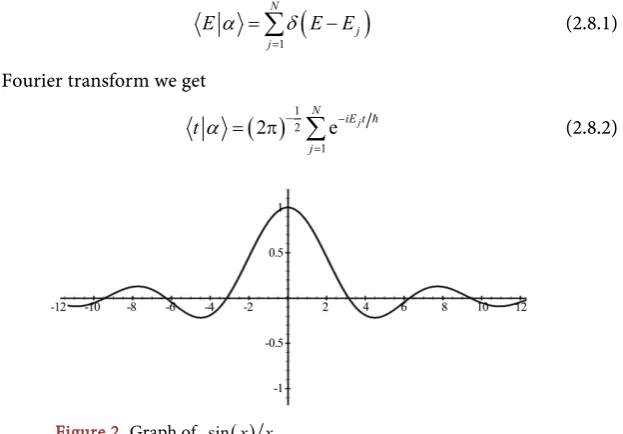
The graph of xα _{has the form (}_{Figure 2}_).

The function xα has maximum value for

x

=

0

, vanishes for

2

x k∆ = ±π_{. It and its squared are equal nearly to half of their maxima for}

2 2

x k∆ π

≈ _or x k∆ ≈ π_.

We may then write that

2

x p x k h

∆ ∆ = ∆ ∆ ≅ π = _(2.7.8)

Becauseh> the relation (2.7.6) is conformed with the uncertainty principle announced by Heisenberg [8] and proven somehow by Kennard [9] in 1927.

2

x p

∆ ∆ ≥_(2.7.9)

Similarly because the couple

(

−1_{E t}_,

)

are reciprocal so as

(

−1_{p x}_,

)

we get

2

t E

∆ ∆ ≥ _(2.7.10)

2.8. Emission of Photons from Atoms Following Bohr

Consider a state α _{which has many stable values for its energy and suppose}

that α is the sum of individual states each of them having only one value of energy or one frequency

(

)

1

N

j j

E α δ E E

=

∑

− _(2.8.1)

By Fourier transform we get

( )

12 1 2 N eiE tj

j

t α − −

=

[image:8.595.229.541.498.715.2]

= π

∑

_(2.8.2)

(9)

so that

( )

(

)

2 1

1

2 N 2cos k j

j k j

t

α

− N E E t

= <

 

= π _ + − _



∑∑

 (2.8.3)

By (2.8.3) we see that the probability for observing α at the instant t is maximal for

, 1,2, , ; 0,1,2,

n

k j k j

h n

t n j k N n

E E ν ν

= = ∀ < = =

− − (2.8.4)

In other word we see that from time to time there may have emission/absor- ption of waves with frequencies

(

)

1

j k h Ek Ej

ν

₌ − ₋ _(2.8.5)

This result accords with the theory on the constitution of atoms and mole-cules of Bohr [10] in 1913.

2.9. Obtaining Permutation Relations between Functions of

Creation and Annihilation Operators

Let A B, be two operators obeying the condition

AB BA I≡ + _(2.9.1)

We have

1

m m m

A B AA AB BA_≡ _≡ ₊mA − _(2.9.2)

because at each time we change AB into BA we must add _Am−1_.

So, let f t

( )

be an entire function and f t′

( )

_{its derivative function we}

clear-ly have

( )

f A B Bf A≡ + f A′ (2.9.3) Now from (2.9.3)

( )

2

( )

2

( )

₂

( )

f A B ≡Bf A B f A B B f A+ ′ ≡ + Bf A′ + f A′′ _(2.9.4)

so that by recursion we get

( )

_{( )}

0

m

k

m m k

k m

f A B B f A

k −

=  

≡ _{ }

 

∑

(2.9.5)

From (2.9.5) we can’t sum over _Bm_{because of the mixed coefficient} m k      

under the summation. After thinking we replace (2.9.5) with the following for-mula

( )

( ) ( )

( )

0 1

!

m _k

k

m m

k

f A B B f A

k

=

≡

∑

_(2.9.6)

so that if g B

( )

is an entire function we get the fundamental identity between operators obeying the sole condition AB BA I− ≡

( ) ( )

( )

_{( )}

( )

_{( )}

0 1

!

k k

k

f A g B g B f A

k

∞

=

≡

∑

(2.9.7)

(10)

( ) ( )

( )

_{( )}

( )

_{( )}

0 1 1

!

k k k

k

f B g A g A f B

k

∞

=

≡

∑

− _(2.9.8)

For examples we have successively

(

)

eαDxX X≡ eαDx +

α

eαDx ≡ X+

α

I eαDx

( )

(

)

eαDxf X e−αDx _≡ f X₊

α

I _(2.9.9)

(

)

2 2

e X e X

x x

D βα βα D X

α

≡

α

+

β

( ) 2 2 2 2 2 2 2 ( )2 12

e Dx X e X e eDx X e X e X I e Dx e e eX Dx

β β β β _α _αβ

α +β _≡ −α α α _≡ − α α + α _≡ β α _(2.9.10)

Defining the creation and the annihilation operators by

(

)

1

2 x x x

a± _≡ D _∓X _⇒a a+ −₋a a− + _≡D X XD₋ _≡I_(2.9.11)

we get from (2.9.8), (2.9.9), (2.9.10),

( ) ( )

( )

0 1 1

!

k k k

k

f a g a g a f a

k

∞

− + + −

=

≡

∑

− (2.9.12)

( )

14 2 2

e e e ,

2

x

a _{f x} _{f x} _{x C}

λ λ

λ± 

λ



= _ + _ ∈  

∓ ∓

(2.9.13)

Closing this paragraph we propose from (2.9.6) the new version of the New-ton’s binomial formula

(

)

0 0

1 _e

! x

r r k k k k r yD r

x

k k

r

x y x y y D x x

k k

∞ ∞ −

= =  

+ = _{ } = =

 

∑

(2.9.14)

3. Obtaining Laws of Wave Optics

3.1. Diffraction by a 3D Object Centered at the Origin of Axis

System

Consider an object occupied a limited domain D in space and represented by the object function which may be discontinuous

( )

1 for &

( )

0 for

D D

f r = r∈D f r = r∉D (3.1.1) From the formula (2.1.4) we see that the coexistence of a wave and this object may be represented by

( )

0

( )

3 2

(

0

( )

)

( )

3 2

(

)

0

ei 2 ei ei 2 ei

D D D

k k

f _r k r= π

∑

FT k rf _r kr = π

∑

f _{k k}− kr

_(3.1.2)

Equation (3.1.2) gives rise to the main theorem in wave optics “Theamplitudeofdiffractionofawave k0

intoawave k bytheformofan object isequalto

( )

2π 3 2 _multiplies _the _Fourier_transform _of _the _object

func-tioncalculatedforthedeviationofthewave-vector

(

k k− 0

)

”.

3.2. Diffraction by Systems of Identical Objects Centered at the

Positions

r

_j

(11)

have

(

)

e j r

( )

D j D

f ₋ ₌ − ∇r f

r r r (3.2.1)

(

)

e j

( )

e i j

( )

D j D D

FTf _{r r}₋ ₌FT − ∇r r f _r ₌ −kr f _k _(3.2.2)

and get a useful formula giving the amplitude of diffraction in some direction

k of a plane wave k0

by a set of identical objects

( )

3 2

(

)

( )

3 2

( )

(

)

2 D j 2 D exp j

j FTf f j i

π

∑

r r− = π ∆k

∑

− ∆kr _(3.2.3)

3.3. Applications

3.3.1. Diffraction of k0 by a Semi Space

The semi space under the plane Oxy is described by the object function

( )

( ) ( ) ( ) ( )

, 1

Oxy

f r =u x u y H z u x− = (3.3.1) From the theorem (2.1.4) we see that

( )

ei0

( )

2

(

( )

)

( )

(

( )

)

ei

Oxy _x _y _z

k

f _r k r = π

∑

δ ∆_k δ ∆_k H − ∆_k kr

_(3.3.2)

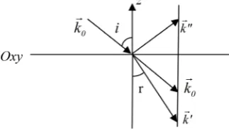
so that there are diffracted waves only for

( ) ( )

0

x y

∆k = ∆k =

0 0 0 0 0

x x y y x x y y

′′− = ′′− = ′− = ′− =

k k k k k k k k (3.3.3) Equations (3.3.3) gives the Descartes law of reflection [11] which implies that

0

k and _k′′_{must be symmetric as shown}_{Figure 3}_{. Moreover if the diffracted}

wave k′ is situated in a medium where the refractive index is n so that

0

k′ =nk _{we get the Snell’s law for refraction}_[11]

(

)

0 0 sin sin 0

x x

k′ −k =k n r− i = _(3.3.4)

3.3.2. Obtaining the Fresnel Formulae

Now, let a a a, ,′ ′′_{denoted the amplitudes of the incident, the refracted and the}

reflected waves; n n1, 2 the upper and lower semi-space refraction indices.

The amplitudes a a′ ′′, _{are proportional to}_a_{and respectively to}

(

0,0,

)

D z

f ∆k′ , f_D

(

0,0,∆k_z′′

)

(3.3.5) Remarking that the Fourier transform of a Heaviside function H z

( )

is

( ) ( )

1 2 1

( )

2

z z

z

H k k

ik

δ

−  

= π _ + π _

 

_(3.3.6)

we get

(

)

(

)

(

)

0 0

0

0 0

sin

cos cos sin

1

2 cos

z

a a a r

a

k r k i k i r

k k

a

a a

k i

k k

ν ν ν

µ µ

′ = = =

′ − −

′ −

′′ = = − ′′ −

(12)

[image:12.595.291.453.73.165.2]

DOI: 10.4236/am.2019.1011064 903 Applied Mathematics Figure 3. Diffraction by the half space under the plane Oxy.

In order to calculate the coefficients μ, ν we will make use of the law of con-servation of energies. The incoming density of energy at the interface Oxy is proportional to _a2_{, to the inclination}

1

cosi and the duration of time an in-coming photon is in the vicinity of it, i.e. to 1

1 v− _or

1

n . Similarly for the density of outgoing energies so that

2 2 2

1 cos 2 cos 1 cos

n a i n a= ′ r n a+ ′′ i_(3.3.8)

The above equations and the formula

(

)

(

)

2 2

4cos sin cos sini i r r=sin i r+ −sin i r− _(3.3.9)

lead by (3.2.3) to the following

(

)

(

)

(

)

(

)

2 2 2 2 2 2 2 2 2

0 1

4k n cos sini i r− =

µ

sin i r− +

ν

sin i r+ −sin i r− _(3.3.10)

• Taken

ν =

0

we get µ =2k n0 1cosi and there is total reflection.

• _Taken µ ν= =2n k_{1 0}cos sini

(

i r−

)

sin

(

i r+

)

we get the Fresnel formulae

[11]

(

)

(

)

(

)

1

1 2

2 cos 2cos sin

cos cos sin

sin

cos cos

cos cos sin

n i

a i r

a n i n r i r

i r

n i n r

a

a n i n r i r

′

= =

+ +

−

′′₌ − _{= −}

+ +

(3.3.11)

• _Taken µ= −νcos

(

i r+

)

_{we get the second Fresnel formulae}_[11]

(

) (

)

(

)

(

)

1

1 2

2 cos 2cos sin

cos cos sin cos

tan tan

n i

a i r

a n i n r i r i r

i r a

a i r

′

= =

+ + −

− ′′

= +

(3.3.12)

From (3.3.12) we find again the Brewster’s condition for total polarization

(

)

2

i r+ = π_, a′′ =0 [11].

3.3.3. Diffraction by a Sphere

The equation of a sphere centered at O and having radius R as shown in Figure 4 is

(

_{, ,}

)

(

2 2

) (

2 2 2

) (

2 2 2 2

)

S x y z =H R −z H R −y −z H R −x −y −z _(3.3.13)

(13)

[image:13.595.191.540.65.735.2]

DOI: 10.4236/am.2019.1011064 904 Applied Mathematics Figure 4. Deflection of waves by a sphere.

(

)

(

) ( )

22 22

(

)

3 2 ₂ ₂ ₂

, , 0,0, 2 2 R e dikz R z d

x y z _R _{R z}

S k k k S k − − z − y R z y

− − −

= = π

_∫

− −

( )

12 2

2 sin

2 R Rk cos

S k Rk

Rk k

−  

= π _ − _

 

_(3.3.14)

As conclusion we see that in a diffraction by a sphere the amplitude of diffrac-tion is inversely propordiffrac-tional to

( )

∆k 2_with ∆ = ∆k k and there is extinction if

tanR k R k∆ = ∆ ⇒ ∆ =R k 0.02_(3.3.15)

Let

ϕ

be the deviation angle in a diffraction as shown Figure 5, we have ex-tinction for

ϕ

such that

0.02 sin

2 2 2 2

k R k

k Rk Rk

ϕ ∆₌ ₌ ∆ ₌

(3.3.16)

For example, for

λ

=10 nm and R=2.5 nm hemoglobin, there is extinc-tion if

0.02

sin 0.0064

2

ϕ ₌ ₌ π

3.3.4. Diffraction of a Plane Wave by Parallel Planes

From (3.2.3) we obtain for example the amplitudes of diffraction of a plane wave by parallel planes perpendicular to Oz at the points ± ±d, 2 , ,d ±Nd as shown

Figure 6

( )

(

)

( )

(

)

(

)

(

)

3 2 3 2

1

sin 2

1

2 e e 2 2 cos

2 _sin ₂

z z

N _z

z ind k ind k n

n _z

Nd k

N d k

d k − ∆ ∆

=

∆

+ ∆

π + = π

∆

∑

(3.3.17)

The maximum amplitudes of diffraction correspond, because k0

and k have opposite projections on Oz as shown Figure 6, to

(

)

0 0

2 cos , 2

2 z

d∆k _{= π ⇒}_m _{d k} _Oz_k ₌ _m_π

(3.3.18)

(

0

)

0 2

2 cosd Oz, 2 sind m m , minteger

k

θ π λ = = =

k (3.3.19)

[image:13.595.307.440.69.181.2]

(14)

[image:14.595.310.439.67.297.2]

DOI: 10.4236/am.2019.1011064 905 Applied Mathematics Figure 5. Angle of deflection.

Figure 6. Diffraction by equidistant parallel planes.

4. Remarks and Conclusions

Someone has said that “Physics is the studies of Nature, how matter and radia-tion behave, move and interact thorough space and time. Mathematics, on the other hand, is logical deductive reasoning based on initial assumption. There are many different systems of mathematics that can describe the same physical phenomenon.” Accordingly this work which improves and completes a previous work [13] is only one attempt for understanding systematically quasi all the principles and hypothesis of quantum mechanics as so as many aspects of wave optics taught in universities. The main remark is that these quantum principles and laws of optics may be deduced from only one simple formula

( ) ( )

3 2

( )

2 ei

k

f _r = π

∑

f _k kr

associated with the property _e±in2π₌₁_{which leads}

to quantization.

May this work brings closer students to modern physics!

Acknowledgements

The author acknowledges Prof. Geneste J.P. for reading and appreciating this work at the World conference on quantum mechanics and nuclear engineering holt in 2019 September at Paris. He thanks warmly the reviewer for giving many judicious remarks and for judging this work as meaningful. He thanks Dr. Feltus Chr. at Luxembourg LIST for laborious writing assistance. He dedicates this work to the Ho Chi Minh-city University of Natural Sciences and the Université libre de Bruxelles where he was formed in the past.

Conflicts of Interest

[image:14.595.314.434.169.291.2]

(15)

References

[1] Planck, M. (1901) Ueber das gesetz der energieverteilung im normalspectrum (On the Law of Distribution of Energy in the Normal Spectrum). Annalen der Physik, 309, 553-560.https://doi.org/10.1002/andp.19013090310

[2] Einstein, A. and Infeld, L. (1938) The Evolution of Physics: The Growth of Ideas from Early Concepts to Relativity and Quanta. Cambridge University Press, Cam-bridge.

[3] de Broglie, L. (1923) Waves and Quanta. Nature, 112, 540. https://doi.org/10.1038/112540a0

[4] Franklina, A. (2013) Millikan’s Measurement of Planck’s Constant. The European Physical Journal H, 38, 572-594.https://doi.org/10.1140/epjh/e2013-40021-3 [5] Pauli, W. (1925) Über den Zusammenhang des Abschlusses der Elektronengruppen

im Atom mit der Komplexstruktur der Spektren. Zeitschrift für Physik, 31, 765-783. https://doi.org/10.1007/BF02980631

[6] Born, M. and Jordan, P. (1925) Zur Quantenmechanik. Zeitschrift für Physik, 34, 858. https://doi.org/10.1007/BF01328531

[7] Griffiths, D.J. (2004) Introduction to Quantum Mechanics. 2nd Edition, Prentice Hall, Upper Saddle River, NJ.

[8] Heisenberg, W. (1927) Über den anschaulichen Inhalt der quantentheoretischen Kinematik und Mechanik. Zeitschrift für Physik, 43, 172-198.

https://doi.org/10.1007/BF01397280

[9] Kennard, E.H. (1927) Zur Quantenmechanik einfacher Bewegungstypen. Zeitschrift für Physik, 44, 326-352. https://doi.org/10.1007/BF01391200

[10] Bohr N. (1913) On the Constitution of Atoms and Molecules. The London, Edin-burgh, and Dublin Philosophical Magazine and Journal of Science, 26, 1-25. https://doi.org/10.1080/14786441308634955

[11] Bruhat, G. (1965) Optique. Masson & Cie,Switzerland.

[12] Do Tan, S. (2019) Advances in Optics, Chapter 5. In: The Fourier Transform Rela-tion between m Dirac bras and Wave Optics, Reviews Book Series, Volume 4, International Frequency Sensor Association Publishing, Barcelona. [13] Do Tan, S. (2018) The Fourier Transform and Principles of Quantum Mechanics.