Linear Regression and Gradient Descent Method for Electricity Output Power Prediction

ISSN Online: 2327-5227 ISSN Print: 2327-5219

DOI: 10.4236/jcc.2019.712004 Dec. 16, 2019 31 Journal of Computer and Communications

Linear Regression and Gradient Descent

Method for Electricity Output Power Prediction

Yuanliang Liao

Tsinghua International School, Campus of Tsinghua High School, Beijing, China

Abstract

Regulating the power output for a power plant as demand for electricity fluc-tuates throughout the day is important for both economic purpose and the safety of the generator. In this work, gradient descent method together with regularization is investigated to study the electricity output related to vacuum level and temperature in the turbine. Ninety percent of the data was used to train the regression parameters while the remaining ten percent was used for validation. Final results showed that 99% accuracy could be obtained with this method. This opens a new window for electricity output prediction for power plants.

Keywords

Machine Learning, Linear Algebra, Linear Regression, Gradient Descent, Error Analysis

1. Introduction

The power output of a power plant typically has a complicated relation with re-spect to the physical parameters, such as temperature, vacuum level, relative humidity, and exhaust steam pressure, etc. [1] [2] [3] [4] [5]. Attempts have been made to resolve the relations using methods such as Bagging algorithm [2], neural network [3], etc. However, either the algorithm itself is complicated or it involves other non-intuitive algorithms such as particle swarm optimization. A simple prediction method without consuming much computing resources is highly desired.

With the advent of computer science, specifically machine learning, methods have been established to build mathematical models based on training data to make predictions or decisions. These methods do not involve explicit programs How to cite this paper: Liao, Y.L. (2019)

Linear Regression and Gradient Descent Method for Electricity Output Power Pre-diction. Journal of Computer and Commu-nications, 7, 31-36.

https://doi.org/10.4236/jcc.2019.712004

Received: November 19, 2019 Accepted: December 13, 2019 Published: December 16, 2019

Copyright © 2019 by author(s) and Scientific Research Publishing Inc. This work is licensed under the Creative Commons Attribution International License (CC BY 4.0).

http://creativecommons.org/licenses/by/4.0/

DOI: 10.4236/jcc.2019.712004 32 Journal of Computer and Communications to perform the task. Using different mathematical algorithms, computers are able to make accurate predictions. Wide applications have been implemented in our daily life, for example, pattern recognition [6] [7], speech recognition [8] [9], text categorization [10] [11], autonomous driving [12] [13], medical diagnosis [14] [15], computational biology [16] [17], etc.

In machine learning, gradient descent is a very popular method for regression. It is an optimization algorithm used to find the values of coefficients of a func-tion that minimizes a cost funcfunc-tion. Gradient descent and cost funcfunc-tion are me-thods and functions that help to analyze sets of data [18] [19]. By combining these two, it enables us to estimate values base on previous records. In this work, we developed a predictive model, that can predict output power of a power plant given the temperature and vacuum level. This is an attempt in using cost func-tion and linear descent after courses of machine learning.

2. Methods

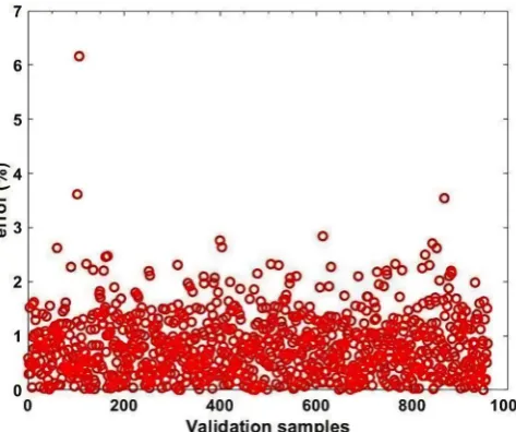
Obtaining the predicted value requires the theta of the linear equation. In order to validate the result, we use ninety percent of the data to predict the result and the remaining ten percent will be used to verify the validity of the predicted data. Graphing will reflect the range of the predicting value. As last, there will be cal-culation of rate of deviation, which is the percent of error comparing the pre-dicted value and actual value.

Linear regression is a linear approach to modeling the relationship between a scalar response or dependent variable and one or more explanatory variables or independent variables. Simply, we have a set of data. Each dependent value cor-responds to another independent variable. We may call these two represent de-pendent variable and indede-pendent variable; our purpose is to find the relation-ship between the dependent variable and the independent variables. Neverthe-less, unlike any “pretty” functions we familiar the most, the variable does not have a direct relationship such as linear or exponential. This can be easily ex-plained: the numbers are authentic data from real life, which means most num-bers will not perfectly match to each other. Because there are many other uncer-tainties in real life, causing the change of dependent variable unstable and with-out pattern, people cannot use equation to explain the relationship of two va-riables. People can, however, plot the data to a graph and draw line of best fit. It looks easy when we usually directly get that by plugging data into excel, but the method of actually drawing the line is not so simple. The word “draw” is not very appropriate because it requires rigid calculations. Assume the linear func-tion is expressed as the following.

( )

h_θ x =θ θ+ x

DOI: 10.4236/jcc.2019.712004 33 Journal of Computer and Communications ( )

( )

1

m

i i

i

hθ x y

=

 ₋ 

 

∑

This simply means the sum of the difference of the estimate value to real val-ue. In order to make it smaller, we take the derivative of the equation and then search for the critical point (1/2 m and square is added for simplifying the cal-culation process):

(

)

( )

J h x y

m x y m θ θ θ θ θ θ θ θ = = ∂ ₌ ∂  _{ − }   _{ }  ∂ _{∂ }  ∂  _{ }  = _{ } + − _{ } ∂  

∑

∑

In addition, we need Gradient Descent to calculate the minimum of the func-tion. Gradient Descent is a formula to find the minimum of a function,

(

)

: , , 0,1

j j i

J j

θ θ θ θ

θ ∂

= − =

∂

For the linear function, we can finally get the slope and the intersection point of the function.

(

)

0 0 1

temp0 ,

i

J

θ θ θ

θ ∂

= −

∂

(

)

1 0 1

temp1 ,

i

J

θ θ θ

θ ∂ = − ∂ 0 temp0 θ = 1 temp0 θ =

3. Results

DOI: 10.4236/jcc.2019.712004 34 Journal of Computer and Communications

Figure 1. Power output versus vacuum level and temperature.

Figure 2. Cost function J decreases with number of iterations.

DOI: 10.4236/jcc.2019.712004 35 Journal of Computer and Communications The difficulty of the program is declaring the data and set the matrix. Because gradient descent and cross validation are only formula. The input of the formula comes from the matrix, which required some manipulation to make the input fit the requirement of the formulas.

4. Conclusion

In this paper, we employed gradient descent method combined with cost func-tion to predict the power output based on the input of vacuum level and tem-perature in a power plant. Less than 1% prediction error has been achieved. Al-though this is a preliminary study, with more complicated gradient method by incorporating more physical parameters, more accurate results could be antic-ipated. Moreover, we believe this method could be extended to other areas.

Conflicts of Interest

The author declares no conflicts of interest regarding the publication of this pa-per.

References

[1] El-Sharkh, M.Y., et al. (2004) A Dynamic Model for a Stand-Alone PEM Fuel Cell Power Plant for Residential Applications. Journal of Power Sources, 138, 199-204.

https://doi.org/10.1016/j.jpowsour.2004.06.037

[2] Tüfekci, P. (2014) Prediction of Full Load Electrical Power Output of a Base Load Operated Combined Cycle Power Plant Using Machine Learning Methods. Interna-tional Journal of Electrical Power & Energy Systems, 60, 126-140.

https://doi.org/10.1016/j.ijepes.2014.02.027

[3] Quan, H., Srinivasan, D. and Khosravi, A. (2013) Short-Term Load and Wind Pow-er Forecasting Using Neural Network-Based Prediction IntPow-ervals. IEEE Transac-tions on Neural Networks and Learning Systems, 25, 303-315.

https://doi.org/10.1109/TNNLS.2013.2276053

[4] Na, M.G., Jung, D.W., Shin, S.H., Jang, J.W., Lee, K.B. and Lee, Y.J. (2005) A Model Predictive Controller for Load-Following Operation of PWR Reactors. IEEE Trans-actions on Nuclear Science, 52, 1009-1020.

https://doi.org/10.1109/TNS.2005.852651

[5] Liu, J., Fang, W.L., Zhang, X.D. and Yang, C.X. (2015) An Improved Photovoltaic Power Forecasting Model with the Assistance of Aerosol Index Data. IEEE Transac-tions on Sustainable Energy, 6, 434-442.

https://doi.org/10.1109/TSTE.2014.2381224

[6] Weiss, S.M., Kapouleas, I. and Shavlik, J.W. (1990) An Empirical Comparison of Pattern Recognition, Neural Nets and Machine Learning Classification Methods. In: Shavlik, J.W. and Dietterich, T.G., Eds., Readings in Machine Learning, Morgan Kaufmann Publishers, San Mateo, 177-183.

[7] Riesen, K. and Bunke, H. (2008) IAM Graph Database Repository for Graph Based Pattern Recognition and Machine Learning. In: Joint IAPR International Work-shops on Statistical Techniques in Pattern Recognition (SPR) and Structural and Syntactic Pattern Recognition (SSPR), Springer, Berlin, Heidelberg, 287-297.

https://doi.org/10.1007/978-3-540-89689-0_33

DOI: 10.4236/jcc.2019.712004 36 Journal of Computer and Communications

Overview. IEEE Transactions on Audio, Speech, and Language Processing, 21, 1060-1089.https://doi.org/10.1109/TASL.2013.2244083

[9] Liu, Y., et al. (2006) A Study in Machine Learning from Imbalanced Data for Sen-tence Boundary Detection in Speech. Computer Speech & Language, 20, 468-494.

https://doi.org/10.1016/j.csl.2005.06.002

[10] Sebastiani, F. (2002) Machine Learning in Automated Text Categorization. ACM Computing Surveys, 34, 1-47.https://doi.org/10.1145/505282.505283

[11] Joachims, T. (1998) Text Categorization with Support Vector Machines: Learning with Many Relevant Features. In: European Conference on Machine Learning, Springer, Berlin, Heidelberg, 137-142.https://doi.org/10.1007/BFb0026683

[12] Dogan, Ü., Edelbrunner, J. and Iossifidis, I. (2011) Autonomous Driving: A Com-parison of Machine Learning Techniques by Means of the Prediction of Lane Change Behavior. IEEE International Conference on Robotics and Biomimetics, Phuket Island, 7-11 December 2011, 1837-1843.

https://doi.org/10.1109/ROBIO.2011.6181557

[13] Sallab, A.E.L., et al. (2017) Deep Reinforcement Learning Framework for Auto-nomous Driving. Electronic Imaging, 19, 70-76.

https://doi.org/10.2352/ISSN.2470-1173.2017.19.AVM-023

[14] Foster, K.R., Koprowski, R. and Skufca, J.D. (2014) Machine Learning, Medical Di-agnosis, and Biomedical Engineering Research-Commentary. Biomedical Engi-neering Online, 13, 94.https://doi.org/10.1186/1475-925X-13-94

[15] Kononenko, I. (2001) Machine Learning for Medical Diagnosis: History, State of the Art and Perspective. Artificial Intelligence in Medicine, 23, 89-109.

https://doi.org/10.1016/S0933-3657(01)00077-X

[16] Ben-Hur, A., et al. (2008) Support Vector Machines and Kernels for Computational Biology. PLoS Computational Biology, 4, e1000173.

https://doi.org/10.1371/journal.pcbi.1000173

[17] Angermueller, C., et al. (2016) Deep Learning for Computational Biology. Molecu-lar Systems Biology, 12, 878.https://doi.org/10.15252/msb.20156651

[18] Zinkevich, M., et al. (2010) Parallelized Stochastic Gradient Descent. Advances in Neural Information Processing Systems, 23, 2595-2603.