Munich Personal RePEc Archive
Multi-Object Auctions with Resale: An
Experimental Analysis
Pagnozzi, Marco and Saral, Krista Jabs
January 2013
Multi-Object Auctions with Resale:
An Experimental Analysis
Marco Pagnozziy Krista Jabs Saralz
January 2013
Abstract
We analyze the e¤ects of resale through bargaining in multi-object uniform-price auctions with asymmetric bidders. The possibility of resale a¤ects bidders’ strategies, and hence the allocation of the objects on sale and the seller’s revenue. Our experimental design consists of four treatments: one without resale and three resale treatments that vary both the bargaining mechanism and the amount of information available in the resale market. As predicted by theory: (i) without resale, asymmetry among bidders reduces demand reduction; (ii) resale increases demand reduction by high-value bidders; (iii) low-value bidders speculate by bidding more aggressively with resale. Therefore, resale induces speculation and demand reduction which reduce auction e¢ciency. In contrast to what is usually argued, resale does not necessarily increase …nal e¢ciency and may not reduce the seller’s revenue. Features of the resale market that tend to increase its e¢ciency also reduce the seller’s revenue.
JEL Classi…cation: D44, C90.
Keywords: multi-object auctions, resale, asymmetric bidders, bargaining, economic exper-iments.
We would like to thank Ciro Avitabile, Vincent Crawford, Dan Levin, Tim Salmon, and Anastasia Semykina for extremely helpful comments, as well as seminar participants at the University of Padova, the University of Verona, the University of Milan Bicocca, the 2011 ASFEE Conference, ESA Chicago-Luxembourg, the CSEF-IGIER Symposium on Economics and Institutions in Anacapri, and the 2nd EIEF-UNIBO Workshop on Industrial Organization. We would also like to thank Webster University Geneva for funding this project.
yDepartment of Economics and CSEF, Università di Napoli Federico II, Via Cintia (Monte S. Angelo), 80126
Napoli, Italy. Email: [email protected].
zGeorge Herbert Walker School of Business and Technology, Webster University Geneva, Route de Collex 15,
1. Introduction
Auctions are often characterized by the possibility of resale by winning bidders, which may dra-matically alter the outcome from what would have been observed without resale. U.S. Treasury
Bills and the Regional Greenhouse Gas Initiative (RGGI) program to sell CO2 allowances are
two economically relevant examples of auctions with an active resale market, and in the latter auction prices are in general lower than resale prices (Zhou, 2011) — a discrepancy that hints at the impact of resale. In spectrum auctions, bidders are typically allowed to trade the licenses acquired, and it is relatively common to observe small bidders winning and then reselling to
larger ones.1
Post-auction resale may exist because of asymmetry in bidders’ valuations (Hafalir and Krishna, 2008; Zheng, 2002), valuations changing after the auction (Haile, 2001, 2003; Gupta and Lebrun, 1999), and potential bidders unable to participate in the auction (Milgrom, 1987). In this paper, however, we will focus on resale emerging because of the strategic choices of bidders in the auction (Garrat and Tröger, 2006; Pagnozzi, 2010).
In fact, in multi-object auctions bidders have an incentive to reduce demand — i.e., bid less than their valuations for marginal units, in order to reduce the auction price and pay less for inframarginal units (Wilson, 1979; Ausubel and Cramton, 1998) — and the possibility of resale exacerbates this incentive since bidders will have a chance to purchase, in the resale market, a unit that they do not acquire in the auction. Moreover, even bidders with low values have an incentive to speculate and bid especially aggressively in an auction if they know they will have a chance to resell the objects acquired. Both speculation and demand reduction make it more likely that the allocation of the objects on sale in the auction will be ine¢cient, and hence that bidders will be willing to trade in a post-auction resale market. So the possibility of resale a¤ects both e¢ciency and the seller’s revenue.
To explore these e¤ects, we theoretically and experimentally examine the impact of resale in multi-object auctions with asymmetric bidders. Speci…cally, we consider a uniform-price auction with two identical units on sale and two bidders, one strong and one weak. The strong bidder has a higher valuation and demands both units; the weak bidder has a lower valuation and demands
only one unit.2 Considering bidders with di¤erent characteristics allows us to distinguish the
di¤erent bidding strategies that they adopt in the auction, and the di¤erent e¤ects that the presence of a resale market has on these strategies. We assume that resale takes place through a post-auction bargaining procedure between bidders, so that bidders share the gains from trade
1For example, in the UK 3.4 GHz auction, two small bidders, Red Spectrum and Public Hub, won one license
each and resold them to Paci…c Century Cyberworks, a much larger company that was considered to have the highest valuation for the licenses on sale in the auction but chose not to outbid its competitors (Pagnozzi, 2010). In the 2000 UK auction, Orange won a 3G mobile-phone license and was later acquired by NTL (a consortium controlled by France Telecom) that participated in the same auction but did not win any license.
2For example, in an auction for geographically di¤erentiated mobile phone licenses, a strong bidder can be
in the resale market, if there are any.
In this context, without resale it is a dominant strategy for a weak bidder to bid up to his valuation for a unit. By contrast, when resale is allowed, a weak bidder speculates by bidding more than his valuation, because winning the auction has the additional option value of providing a chance of reselling to the strong bidder (Haile, 2003; Garratt and Tröger, 2006; Pagnozzi, 2007).
Our theoretical analysis also shows that, although strong bidders may bene…t from a demand reduction strategy that reduces the auction price, asymmetry among bidders’ valuations reduces the incentive to reduce demand, because it is more costly to lose an object for a bidder with a higher valuation, and less costly to outbid a competitor with a lower valuation. Without resale, strong bidders with relatively high valuations outbid weak bidders and win both units; while strong bidders with relatively low valuations reduce demand for the second unit and allow the weak bidder to win one unit. The presence of resale, however, may dramatically change this result: resale makes demand reduction more attractive for strong bidders, because it provides them with a second opportunity to purchase a unit not acquired in the auction. Accordingly, with resale, strong bidders always reduce demand, regardless of their valuations (Pagnozzi, 2009, 2010).
In order to both test and inform the theory of multi-object auctions with resale, we
con-ducted a series of controlled laboratory experiments with four treatments: No Resale,Complete
Information Resale,Incomplete Information Resale, and Bargain.The no resale treatment con-sisted of subjects only participating in an ascending auction. The complete information and the incomplete information resale treatments involved a secondary market after the auction where one of the two bidders was randomly chosen to make a take-it-or-leave-it o¤er to the other
bid-der.3 In the …rst of these treatments, subjects were given complete information regarding the
competitors’ values in the resale market, while in the second, information was restricted to the distribution of the competitors’ values. In the bargain treatment, we extended the incomplete information resale treatment to an unstructured bargaining game where both subjects were al-lowed to make multiple o¤ers and to communicate through computerized chat during the resale
stage.4
We analyze di¤erent resale mechanisms in order to investigate how the outcome of the resale market, and its e¤ects on bidders’ strategies in the auction, depend on the speci…c procedure adopted by bidders to trade after the auction. The complete and incomplete information resale treatments consider a static and more structured resale market, where each bidder expects to be given full bargaining power with equal probability. The bargain treatment extends this simple
3This resale mechanism was analyzed by Calzolari and Pavan, 2006.
4Feltovich and Swierzbinski (2011) use a similar approach with computerized chat in an unstructured
environment in an attempt to replicate a more ‡exible, and arguably more realistic, post-auction bargaining procedure among auction bidders. To the best of our knowledge, we are the …rst to consider an unstructured bargaining procedure to experimentally analyze post-auction resale markets.
Consistent with the theoretical predictions, we show that in the no resale treatment weak bidders bid up to their value. This result parallels earlier work in single unit ascending auctions
(e.g., Coppinger et al., 1980; Kagel et al., 1987), and con…rms the robustness of value bidding
in the multi-object context.5 We also …nd that the addition of a resale market signi…cantly
increases weak bidders’ bids, indicating speculation, regardless of the speci…c structure of the resale market.
Also consistent with the theoretical predictions on demand reduction, in the no resale treat-ment strong bidders drop out at low prices with much higher frequency when their valuation is relatively low. This complements previous experimental results that have shown the prevalence
of demand reduction in ascending auctions when bidders are symmetric (e.g., Alsemgeest et
al., 1998; Kagel and Levin, 2001, 2005; Engelmann and Grimm, 2009; Goeree et al., 2012):6
strong bidders do engage in demand reduction, but value asymmetry between bidders tends to reduce demand reduction when resale is not allowed. By contrast, with resale strong bidders reduce demand regardless of their valuations, by dropping out at very low prices and they do so signi…cantly more than without resale, especially if they have high values. The largest amount of demand reduction occurs in the complete information resale and bargain treatments.
Comparing the di¤erent resale treatments, the incomplete information treatment generated higher uncertainty of the resale outcome, because it involved a less ‡exible trading mechanism with lower information for subjects. As a result, strong bidders tended to reduce demand less than in the bargain and the complete information resale treatments. Moreover, weak bidders tended to speculate less in the incomplete information and bargain resale treatments than in the complete information resale treatment, because they correctly expected to obtain higher resale pro…t in the latter.
In summary, as predicted by theory, our experimental analysis shows that asymmetry and resale a¤ect bidders’ strategy in an auction: (i) without resale strong bidders reduce demand much less often when they have high valuations; (ii) the possibility of resale increases demand reduction by strong bidders; (iii) weak bidders bid more aggressively when they have a chance to resell.
Beyond the results speci…cally related to bidding, our experiments also allow us to analyze the e¤ect of post-auction resale on e¢ciency and the seller’s revenue. It is often argued that
5McCabeet al., (1990) also provide evidence of value bidding for bidders with single-unit demand in
multi-unit ascending auctions. See Kagel (1995) for a comprehensive overview of experimental data on value bidding in single-unit auctions. Also see Kagel and Levin (2011) and Kwasnica and Sherstyuk (2012) for a broad survey of more recent experimental results in multi-object auctions.
6The literature shows that demand reduction, although present in various types of multi-object auctions, is
resale after an auction should always be allowed, because it always increases e¢ciency by allowing bidders to trade, if they are willing to do so, in the presence of gains from trade. But our analysis suggests that this is not necessarily the case. Although resale does increase e¢ciency after the auction, it also has a signi…cant e¤ect on bidders’ strategies during the auction, and these tend to reduce auction e¢ciency. In fact, in all resale treatments auction e¢ciency is lower than in the treatment without resale. Yet, the net e¤ect is ambiguous: in the incomplete information resale treatment, …nal e¢ciency is not signi…cantly di¤erent from …nal e¢ciency without resale; while in the two other resale treatments …nal e¢ciency is higher.
The net e¤ect of resale on revenue is also ambiguous. In theory, allowing resale should always reduce the seller’s revenue, because it should induce strong bidders to reduce demand, thus reducing the auction price, possibly down to zero (or to the reserve price, if one is present). Our experimental results, however, indicate that allowing resale increases the seller’s revenue when strong bidders do not reduce demand, since weak bidders bid more aggressively with resale than without, thereby increasing the auction price. On balance, the seller’s revenue in the treatment without resale is not signi…cantly higher than in the treatment with resale under incomplete information, but it is signi…cantly higher than either the bargain or the complete information resale treatment.
We also analyze how the e¢ciency of the resale market depends on the resale mechanism adopted by bidders. A more ‡exible bargaining mechanism and more precise information about the size of the gains from trade increase the probability of successful resale and the resulting …nal e¢ciency. With take-it-or-leave-it o¤ers in the resale market, the probability of successful resale is higher when weak bidders choose the resale price, since they tend to make less aggressive o¤ers that are more likely accepted. However, all of these factors also reduce the seller’s revenue in the auction because, by increasing the e¢ciency of the resale market, they increase strong bidders’ incentive to reduce demand. So there is a trade-o¤ between higher …nal post-resale e¢ciency and higher revenue in the auction.
The resale price depends on the resale mechanism and is higher when bidders have more information in the resale market, because in this case the resale seller (weak bidder) manages to obtain higher pro…ts. However, the resale pro…t of the resale seller is lower than that of the resale buyer (strong bidder) in all resale mechanisms. Considering also the auction pro…t, weak bidders always obtain higher total pro…ts when resale is allowed, while strong bidders may obtain lower total pro…ts with resale, depending on the actual resale mechanism. Finally, our analysis shows that resale prices tend to be higher than auction prices, since intra-bidder resale takes place when strong bidders reduce demand to allow weak bidders to win, thus reducing the
auction price below the competitive level.7
Our paper contributes to the recent experimental literature on auctions with resale.
Exper-7This is consistent with the evidence from various actual auction markets. For example, in the New Zeland
iments on single-object auctions with resale include Georganas (2011), Georganas and Kagel
(2011), Langeet al. (2011), Saral (2012) — that test how the presence of a resale market a¤ects
bidding behavior — and Harstad (2012) — that analyzes the e¤ects of aftermarkets on e¢ciency. In these papers resale takes place either automatically, through another auction, or through a
take-it-or-leave-it o¤er by the auction winner. Filiz-Ozbayet al. (2012) provide the only other
experimental analysis of multi-object auctions with resale that we are aware of. They consider the e¤ects of complementarities in comparing the e¢ciency of a Vickrey auction and indepen-dent second-price auctions and assume that, in the resale market, the auction winner makes take-it-or-leave-it o¤ers to the losers, separately for each object acquired. Hence, the results of
Filiz-Ozbay et al. (2012) complement ours, since they focus on the e¤ects of a speci…c resale
mechanism on di¤erent auction formats, in the presence of more complex bidders’ valuations. The rest of the paper is organized as follows. Section 2 presents a theoretical analysis of the model that we refer to for our experimental design, and its predictions in terms of bidding strategies, e¢ciency and the seller’s revenue. Section 3 discusses the design of our experiments, and Section 4 presents the experimental results. Speci…cally, Sections 4.1 and 4.2 shows bidding behavior by weak and strong bidders respectively, Section 4.3 discusses e¢ciency and the seller’s revenue, and Section 4.4 analyzes subjects’ behavior in the resale market. Finally, Section 5 concludes with a summary and discussion of our results. The Appendix contains sample instructions and screenshots from our experiments.
2. Model and Theoretical Predictions
We construct the simplest possible model that will allow us to experimentally investigate the e¤ects of resale on bidding strategies by asymmetric bidders, and on their incentives to reduce demand and speculate.
Auction. There is a (sealed-bid) uniform-price auction for 2 units of an identical good, where the reserve price is normalized to zero: each player submits 2 non-negative bids, one for each of the units; the 2 highest bids are awarded the units; and the winner(s) pay a price equal to the
3rd-highest bid for each unit won. We consider a uniform-price auction because it is the auction
mechanism in which the incentive to reduce demand arises more clearly and because it is widely
used to allocate multiple objects.8 The qualitative results of the analysis, however, also hold
for any mechanism to allocate multiple units in which players face a trade-o¤ between winning more units and paying lower prices. The auction may be followed by a resale market.
Bidders and Valuations. There are 2 risk-neutral asymmetric bidders. Bidders di¤er both in the number of units that they demand, and in their valuations for those units. Speci…cally, bidder
S, the strong bidder, demands 2 units and has valuation vS U vS;vS for each unit on sale
8Of course, the uniform-price auction is not an optimal mechanism in our context, neither with resale nor
(i.e., he has ‡at demand);9 bidder W, theweak bidder, demands 1 unit only and has valuation
vW U vW;vW for that unit. Bidders are privately informed about their valuations, which
are independent. We assume that vS vW, so that bidder S always has a higher valuation
than bidder W, and bidders know the ex-post e¢cient allocation of the units on sale before
the auction. For simplicity, we also assume that bidder W cannot win more than 1 unit in the
auction, even if resale is allowed.
Our assumption on bidders’ valuations ensures that in our experiments bidders know the role they will have in the resale market when they bid in the auction — i.e., whether they will have a chance to buy or sell in the resale market — allowing us to focus on the di¤erent bidding strategies of the two types of bidders and on how these strategies are a¤ected by the possibility of resale. The assumption also implies that bidders know there are gains from trade in the resale
market ifW wins a unit.
Resale Market. When resale is allowed after the auction, if bidder W wins a unit he can resell
it to bidder S. In contrast to previous experiments on auctions with resale that assume a
more restricted structure for the resale market,10 we assume that resale takes place through
bargaining between bidders. We believe that this is a more realistic representation of many real-life situations in which bidders attempt to trade after an auction but do not follow a formal trading mechanism (e.g., because no bidder has the bargaining power to impose his preferred trading mechanism) and may be unable to trade even if they know there are mutual gains from doing so (e.g., because of incomplete information).
When they bid in the auction, both bidders expect to obtain some share of the gains from
trade in the resale market. The actual gains from trade in the resale market arevS vW (since
W’s outside option when he trades in the resale market is equal to his valuation, while S’s
outside option is zero). In order to capture di¤erent bargaining mechanisms, we assume that
bargaining in the resale market results in S obtaining a share of the gains from trade and W
obtaining a share1 of the gains from trade. This can be interpreted as bidders trading at a
resale price
r vW + (1 ) (vS vW) = vW + (1 )vS:
Our results are robust to many alternative models of the resale market and hold forany sharing
of the gains from trade in the resale market that is individually rational for bidderW (i.e., such
that the resale price is not lower than W’s valuation).11
9All our qualitative results also hold in the presence of complementarities, although bidderS’s incentive to
reduce demand is lower in this case, if there is a chance that he may not manage to acquire the second unit in the resale market.
1 0Georganas (2011) and Harstad (2012) use a secondary auction for the resale market, while Georganas and
Kagel (2011) and Filiz-Ozbayet al. (2012) utilize take-it-or-leave it o¤ers by the auction winner. Lange et al.
(2011) and Saral (2012) assume automatic transfers to bidders with higher valuations.
1 1All our results also hold if the resale market is not necessarily e¢cient — for example, if bidders fail to trade
In our experiments, we consider di¤erent bargaining mechanisms for the resale market. In
one mechanism, if bidderW wins a unit in the auction, bidders are allowed to freely bargain over
the resale price (see Section 3). In another mechanism, one of the two bidders, chosen randomly, is given the possibility of making a take-it-or-leave-it o¤er to the other bidder (Calzolari and
Pavan, 2006). This second resale mechanism, in which in expectation bidders obtain 12 of the
expected gains from trade in the resale market, is a special case of our class of bargaining
mechanisms, when = 12.
Bidding Strategies. There isdemand reduction if a bidder bids less than his valuation for a unit,
while there isspeculation if a bidder bids more than his valuation for a unit. In a uniform-price
auction without resale, it is a weakly dominant strategy for a bidder to bid his valuation for the
…rst unit, exactly as in a single-object second-price auction. Yet, bidderSmay …nd it pro…table
to reduce demand and bid less than his valuation for the second unit in order to pay a lower price for the …rst unit in case he loses the second, thus obtaining a higher pro…t. The logic is the same as the standard textbook logic for a monopsonist withholding demand: buying an additional unit increases the price paid for the …rst, inframarginal, units. Moreover, when resale
is allowed, bidderW may …nd it pro…table to speculate and bid more than his valuation in the
auction, if he expects to resell the item at a price higher than his valuation in the resale market.
Of course, the auction allocation is ine¢cient when bidderW wins a unit in the auction (because
he speculates or because bidderS reduces demand).
We will now describe the equilibrium bidding strategies with and without resale. Because our model has 2 units on sale and a total demand for 3 units, to characterize bidding strategies
it will be su¢cient to describeW’s bid for one unit, andS’s bid for the second unit. The lowest
of these two bids will be the auction price, and either S will win both units on sale at a price
equal toW’s bid, or the two bidders will win one unit each at a price equal to S’s bid.
2.1. Auction without Resale
Consider an auction without resale. Without resale, it is a weakly dominant strategy for bidder
W to bid his valuation for a unit — i.e., vW.12 Given this strategy, bidder S has a choice
between two alternatives. First, by outbidding W in the auction, S can win two units at an
expected price equal to E[vW], thus obtaining a pro…t equal to2 (vS E[vW]). Second, S can
reduce demand and bid 0 for the second unit, thus winning one unit at price 0 and letting W
win the other unit.13 In this case,S obtains a pro…t equal tovS 0. Therefore, bidderSprefers
to reduce demand and win one unit only rather than outbid bidder W if and only if
vS >2 (vS E[vW]) , vS<2E[vW]:
1 2IfW wins the auction at price p, he earns(v
W p), while ifW loses the auction, he earns 0. So he bids a price such that his pro…t from winning is equal to zero.
When resale is not allowed, bidder S’s incentive to reduce demand in the auction is lower when he has a relatively high valuation, because reducing demand and not winning the second
unit is more costly when that unit is more valuable, or when he expects bidderW to have a low
valuation and hence to bid less aggressively, because outbidding bidder W to win the second
unit is less costly. Accordingly, without resale, if vS <2E[vW]bidder S and bidder W win one
unit each and the auction price is equal to 0; ifvS >2E[vW]bidder S wins both units and the
auction price is equal to vW.
2.2. Auction with Resale
Consider an auction with resale. When resale is allowed, a player’s “willingness to pay” for a unit in the auction — i.e., the highest auction price that a player is happy to pay for a unit — is represented by the price at which he expects to buy or sell a unit in the resale market (e.g., Milgrom, 1987).
By assumption, if bidder W wins a unit in the auction, he obtains an actual surplus equal
to(1 ) (vS vW) in the resale market. Therefore, bidderW bids
vW + (1 )E[vS vWjvW] = vW + (1 )E[vS]
for a unit on sale in the auction.14 Notice that this can be interpreted asE[rjvW], the price at
which bidder W expects to sell to bidder S in the resale market. Bidder W speculates because
of the option to resell to bidderSand bids higher than his valuation for a unit, and hence higher
than without resale.
Since bidder W bids his expected resale price in the auction, bidderS has a choice between
two alternatives. First, bidder S can outbid bidder W and win 2 units in the auction at an
expected auction price equal to
E[E[rjvW]] = E[vW] + (1 )E[vS];
thus obtaining an expected pro…t equal to
2 (vS E[vW] (1 )E[vS]): (2.1)
Second, bidder S can reduce demand and bid zero for the second unit in the auction, thus
winning one unit at price 0 in the auction and then buying the second unit from bidder W in
resale market at an expected resale price equal to
E[rjvS] = E[vW] (1 )vS:
1 4If W wins a unit in the auction at price p, he obtains an expected pro…t equal to v
W p +
In this case, S obtains an expected total pro…t equal to15
vS 0
| {z }
auction pro…t
+vS E[rjvS]
| {z }
resale pro…t
= (1 + )vS E[vW]: (2.2)
Comparing (2.1) and (2.2), bidderS prefers to reduce demand in the auction when resale is
allowed if and only if
(1 ) (2E[vS] vS) + E[vW]>0 , (1 ) vS+vS vS + E[vW]>0:
Since this inequality is always satis…ed, bidder S always prefers to reduce demand when resale
is allowed.16 Notice that this result holds for every and for every v
S. Basically, bidder S
is willing to bid a much lower price in the auction because of the option to buy in the resale
market. And demand reduction allows bidderS to win 1 unit at price 0 in the auction and then
purchase the other unit from bidderW at pricer in the resale market, rather than pay bidder
W’s expected resale price for both units in the auction. The …rst option is more attractive than
the second (unless bidder S expects the resale price to be much higher than bidder W, which
can be the case whenvS is very high compared to its ex-ante expected value — see footnote 16
— but this never happens when bidderS’s valuation is uniformly distributed).
As a result, when resale is allowed, S andW win one unit each and then trade in the resale
market. The auction price is equal to 0. (Of course, this can also be interpreted as tacit collusion among bidders, intended to reduce the seller’s revenue.)
Summing up, the theoretical predictions of the model that we test using experimental methodology are the following.
Result 1. Without resale, bidder W bids vW and bidder S reduces demand if and only if
vS <2E[vW].
Result 2. With resale, bidder W bids above vW and bidder S always reduces demand.
Result 3. The allocation of the units on sale in the auction is always ine¢cient with resale, but not necessarily without resale. The …nal allocation of the units on sale (after resale) is always e¢cient with resale, but not necessarily without resale.
Result 4. The seller’s revenue is always equal to zero with resale, but not necessarily without resale.
1 5Notice that bidderS’s expected pro…t from resale can also be interpreted as
E[vS vWjvS], his share of the expected gains from trade in the resale market.
1 6More generally — i.e., when bidders’ valuations are not necessarily uniformly distributed — a su¢cient
(but not necessary) condition for bidder S always preferring to reduce demand when resale is allowed is that
3. Experimental Design
The experiment was designed around three primary objectives: (i) analyze bidding behavior in
uniform-price multi-object auctions with asymmetric bidders and no resale; (ii) analyze how
post-auction resale between bidders a¤ects their bidding strategies, e¢ciency, and the seller’s
revenue;(iii)investigate how auction bidders trade in the resale market, and how their strategies
are a¤ected by di¤erent resale mechanisms.
We implemented four treatments, one without resale, and three with di¤erent resale mech-anisms. The resale mechanisms were designed to evaluate the e¤ects of di¤erent levels of infor-mation in the resale market on bidders’ strategies in the auction, and to check the robustness of our qualitative results to di¤erent trading procedures in the resale market. Each session of the experiment consisted of a single treatment, and the recruitment process restricted subjects’ participation to a single session. At the beginning of a session subjects were randomly assigned to either the role of weak or strong bidder and that role assignment remained constant for the duration of the experiment.
In all treatments, each period began with an ascending clock uniform-price auction for two
items of a hypothetical good. Each auction always had 1 strong bidder and 1 weak bidder.17
The strong bidder was allowed to purchase up to 2 units of the hypothetical good, and randomly
drew his private valuation for each unit from a uniform distribution on the range[30;50]. The
weak bidder could purchase 1 unit only, and randomly drew his private valuation from a uniform
distribution on the range [10;30]. Throughout the instructions and the experiment, the strong
bidder was referred to as a 2-unit bidder and the weak bidder as a 1-unit bidder to minimize labeling e¤ects. During the auction each bidder was given information about the distribution of his competitor’s valuation and about the number of units he demanded.
Bidders participated in the auction through a computer interface where they were able to see a bid clock gradually increasing from 0 in increments of 1, which indicated the auction price for a unit. To bid in the auction, subjects chose to “drop out” when the clock reached a price at which they wanted to exit the auction. The auction ended as soon as one bidder dropped out, and the auction price paid for each unit was equal to the dropout bid. If neither subject dropped out, the auction ended when the bid clock hit the maximum possible value of the strong bidder, 50, and the units were awarded by random draw. If both subjects dropped out simultaneously, ties were again broken randomly by the computer program. If a bidder won a unit, he earned the di¤erence between his value and the price resulting from the auction.
In the treatment without a resale market, the auction determined the …nal outcome. In the three resale treatments, if the weak bidder won a unit, there were gains from trade between bidders and the resale market immediately started with the same participants from the auction. Two of the three resale treatments involved a take-it-or-leave-it o¤er where the proposer was
1 7We use ascending auctions (rather than sealed-bid ones) because they are widely used in the …eld and, based
determined with 50/50 probability. If the weak bidder was selected as the proposer, he had the opportunity to o¤er a buy price to the strong bidder, who could then accept or reject the o¤er. Correspondingly, if the strong bidder was selected as the proposer, he had a chance to o¤er a sell price to the weak bidder, who could then accept or reject the o¤er. Neither of these two treatments allowed communication between the resale participants and the sole di¤erence involved the amount of information conveyed to the participants. In the …rst case, complete information of the competitor’s valuation was provided to each participant after the auction while in the second, the information provided was limited to the distribution of the competitor’s valuation.
The third and …nal resale treatment relaxed the no communication and one-shot o¤er con-straints by implementing an unstructured bargaining game where both the weak and strong bidder could simultaneously make o¤ers through a computerized o¤er board. Only one posted o¤er per participant was allowed at a time, but o¤ers could always be changed prior to agree-ment. Either role could accept the o¤er made by their resale counterpart and the resale stage terminated once an o¤er was accepted. Throughout the resale stage, bidders could also send each other messages and discuss the o¤ers through an anonymous chat. Bidders had a time
limit of 3 minutes to reach agreement.18
In all resale treatments, either participant had a choice to exit the resale market without trading at any point of their choosing. If a resale o¤er was agreed upon, the unit was transferred from the weak bidder (seller) to the strong bidder (buyer). The weak bidder earned the di¤erence between the resale price and his value, and the strong bidder earned the di¤erence between his value and the resale price. If resale failed, both bidders earned 0. Any resale earnings were in addition to the earnings from the auction. The experimental treatments are summarized below.
1. No Resale: Subjects only participated in the auction.
2. Complete Information Resale (Comp Resale): After the auction, if the weak bidder won a unit, one of the bidders was randomly chosen to make a take-it-or-leave-it o¤er to the other and both bidders were given complete information regarding the valuation of the competitor.
3. Incomplete Information Resale (Incomp Resale): This treatment was identical to the complete information resale treatment, except that in the resale stage bidders’ valuations were not revealed to the competitors and the o¤er proposer was given a calculator tool (slide bar of potential o¤ers) to determine the probability that his o¤er led to negative resale earnings for the responder.
1 8This was not an overly binding constraint. In the bargain treatment we observe 351 resale markets with 44
4. Bargain: After the auction, if the weak bidder won a unit, both bidders were allowed to make and accept o¤ers and to communicate via anonymous computerized chat in an unstructured bargaining game.
We conducted 3 sessions for each treatment yielding a total of 12 sessions. The no resale, complete information resale, and incomplete information resale sessions each consisted of 30 periods. The bargain treatment required more time for each auction/resale round because of the nature of the resale stage, so each session of this treatment consisted of 20 periods. To ensure the least amount of changes possible we used the exact same value draws across all sessions. We had 16 participants in each session, which were randomly assigned to the roles of weak and strong bidder (8 subjects per role). The subjects were students at Florida State University and were recruited using ORSEE (Greiner, 2004). All sessions were conducted at the xs/fs laboratory in March and June, 2011, and October, 2012.
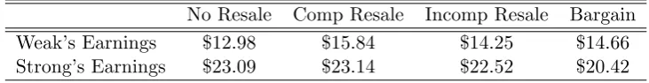
The experiment was programmed using Z-tree software (Fischbacher, 2007), and prior to the beginning of the paid periods, all subjects were given instructions which included two examples of bidding behavior and, in the resale treatments, resale market outcomes. To ensure subjects’ understanding, they were required to correctly complete a computerized quiz before continuing. Payo¤s during the experiment were denominated in experimental currency units, ECUs, which transformed into US dollars at the rate of $0.01 per ECU. Table 3.1 shows the earnings broken down by type and treatment.
No Resale Comp Resale Incomp Resale Bargain
Weak’s Earnings $12.98 $15.84 $14.25 $14.66
[image:14.595.115.481.422.469.2]Strong’s Earnings $23.09 $23.14 $22.52 $20.42
Table 3.1: Average earnings.
4. Experimental Results
In this section, we describe the main results of our experiments. We begin in Sections 4.1 and 4.2 by describing the bidding behavior of weak and strong bidders, respectively, Section 4.3 discusses e¢ciency and the seller’s revenue, while Section 4.4 concludes with subjects’ behavior in the resale market. All data from all periods is included in the following analysis, unless explicitly noted.
4.1. Weak Type Bidding
0 10 20 30 40 50 b id
10 15 20 25 30
v alue No Resale 0 10 20 30 40 50
10 15 20 25 30
v alue Comp Resale 0 10 20 30 40 50 b id
10 15 20 25 30
v alue Incomp Resale 0 10 20 30 40 50
10 15 20 25 30
v alue
[image:15.595.83.545.93.423.2]Bargain
Figure 4.1: Weak Bidding– weighted scatterplot of observed bids (dropouts) by weak bidders
versus valuations in the four treatments.
in the four treatments.19 In all scatterplots, the markers are weighted by the frequency with
which each value/bid combination was observed, so that larger markers indicate more frequent combinations. A line is included to indicate bids equal to values — i.e., the weak bidder’s theoretical bidding function without resale. Bids above (below) this line are higher (lower) than value.
It is clear from the scatterplot that in the no resale treatment (upper left graph of Figure 4.1) the majority of observed bids by weak bidders are equal to value. Quantifying this, we …nd that the mean absolute deviation of bid from value is 0.80 and 83% of observed bids fall within +/-2 of value. For a more accurate test of value bidding, Table 4.1 presents panel random e¤ects
bid regression results on observed bids for the no resale treatment.20 Supporting the theoretical
prediction of value bidding, in the regression model the estimated coe¢cient on the value of the
1 9The …gure only represents observed bids. Because the experiments were based on ascending auctions, we do
not observe the weak bidder’s bid when he wins a unit in the auction.
weak bidder, 0.982, is not signi…cantly di¤erent from 1 (p = 0:689), while the constant is not signi…cantly di¤erent from zero.
Weak Bid Coe¢cient
(robust std. error) p-value
Constant 0:172
(1:150)
0:881
vw 0:982
(0:044) <0:001
Table 4.1: Random e¤ects panel regression - Weak bidding.
The strong adherence of weak bidders’ behavior to the theoretical prediction under no resale conditions parallels previous experimental results of value bidding in ascending auctions (see,
for example, McCabeet al., 1990, and Alsemgeestet al., 1998).
Empirical Result 1: Without resale, weak bidders bid up to their valuations.
In the resale treatment with complete information (the upper right graph of Figure 4.1), it is also clear that the addition of a resale market dramatically changed bids in the upward direction. A Wilcoxon-Mann-Whitney (WMW) test con…rms this di¤erence in observed bids between the
no resale and complete information resale treatments (p < 0:001), providing empirical support
for Result 2.
Many of the observed bids, while certainly higher than value, still lie at or below 30 — the lowest possible value of the strong bidder. A plausible explanation is that since weak bidders only had information regarding the competitor’s value distribution, they may not have wanted
to risk paying more than strong bidders’ valuations.21 This is only a partial story, however,
since the scatterplot only contains observations for auctions where the weak bidder did not win a unit.
In the resale treatment with incomplete information (the lower left graph of Figure 4.1), more weak bidders chose to bid value than under complete information, yet they are also fre-quently bidding above value as predicted by Result 2. However, the above-value bids under incomplete information appear conservative as the majority fall below 30 and we observe more losing bids than under complete information. Arguably, higher uncertainty about the outcome of the resale market and the resale pro…t induced weak bidders to bid less aggressively with incomplete information. Despite this more conservative speculation, we still …nd signi…cant di¤erences in observed bids between the no resale treatment and the incomplete information
resale treatment (p <0:001) and fail to …nd a signi…cant di¤erence between the incomplete and
complete information resale treatments (p= 0:240).
Notice that the graph for the incomplete information resale treatment contains more obser-vations than the bargain and the complete information resale treatments and fewer obserobser-vations
2 1For experimental analysis on the role of expectations in bidders’ deviations from equilibrium strategies see
than the no resale treatment, because weak bidders won more often in the bargain and the complete information resale treatments and less often in auctions without a resale opportunity. As we will show in Section 4.2, this is a consequence of the strong bidders’ strategic behavior.
The …nal resale treatment, bargain (lower right graph of Figure 4.1), resulted in the majority
of bids at value or above.22 This treatment appears to result in fewer aggressive bids, and
relatively more bids at value, especially when contrasted with resale under complete information. The lack of aggressiveness in observed bids is con…rmed by a WMW test that shows no signi…cant
di¤erence between bargain and no resale (p= 0:221), and signi…cant di¤erences between bargain
and either incomplete information resale or complete information resale (p 0:001).23
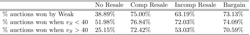
By Results 1 and 2, strong bidders should always let weak bidders win with resale, but without resale they should only let weak bidders win if their unit value is less than 40. Table 4.2 provides the relative frequency of weak bidders winning a unit, overall and broken down by the strong competitor’s value. Resale did result in the weak bidder winning a unit with higher frequency than without resale, with the highest frequency obtained in the complete information resale and bargain treatments. Even with resale, especially in the incomplete information resale treatment, the weak bidder won a unit more often when the strong bidder had a value lower than 40.
No Resale Comp Resale Incomp Resale Bargain
% auctions won by Weak 38.89% 75.00% 63.19% 73.13%
% auctions won when vS<40 51.98% 76.84% 72.03% 74.09%
[image:17.595.90.511.375.435.2]% auctions won when vS>40 25.15% 72.42% 53.03% 70.59%
Table 4.2: Relative frequency of weak bidders winning 1 unit.
Formalizing the above results, table 4.3 presents random e¤ects tobit regression results on bids for weak types. The use of a tobit model is appropriate because of the large number of unobserved bids which are censored at the auction price whenever the weak bidder won a unit in
the auction. We report marginal e¤ects in addition to the tobit model estimates.24 The variable
vW represents the weak bidder’s valuation, while Comp Resale, Incomp Resale, and Bargain are
treatment dummies representing the resale treatments. The no resale treatment serves as our baseline group and the variable Period, which tracks the period of play, is included in Model 2
2 2We include the plus marker in the bargain treatment scatterplot to indicate the dropout bids placed by a
single subject assigned to the weak role who consistently bid at 0 and 1 for the duration of the experiment. This subject’s bidding behavior is exceptional given the overall pattern of the data and is di¢cult to rationalize, so while this subject’s data is included in all of the analysis and graphs that follow, we mark these observations in the scatterplot as outliers.
2 3As the bargain treatment was run with fewer periods than the other three treatments (20 vs. 30 periods per
session), we have also conducted WMW tests on a restricted sample with 20 periods of data for each treatment. All signi…cance results are the same for the restricted sample comparisons.
2 4Our form of the model may also be referred to as a censored normal regression model as the censoring point
may change in each observation (Wooldridge, 2001). Our reported marginal e¤ect = @E[bidj@xbid>price]
to test for learning e¤ects over time.25
(1) (2)
Weak Bid Coe¢cient Marginal
E¤ect
Coe¢cient Marginal
E¤ect
Constant 0:870
(1:444) (11::064484)
vw 0:993
(0:053) 0:659 0:(0993:053) 0:659 Comp Resale
(Comp)
13:248
(2:285) 8:793 13(2:245:282) 8:788 Incomp Resale
(Incomp)
6:951
(2:162) 4:613 6:(2939:160) 4:604
Bargain 6:747
(2:545) 4:478 6:(2665:547) 4:422
Period 0:013
(0:023) 0:008
vw Comp 0:316
(0:092) 0:209 0(0:318:092) 0:211
vw Incomp 0:117
(0:084) 0:077 (00:084):117 0:077
vw Bargain 0:236
(0:108)
0:157 0:236
(0:108)
[image:18.595.152.446.114.345.2]0:157
Table 4.3: Random e¤ects panel tobit - Weak bidding.
The results of Model 1 demonstrate a strong positive e¤ect on weak bidders’ bids when resale is possible, regardless of the form, con…rming Result 2. While all three resale treatments result in speculation by weak bidders, the strength of this e¤ect is strongest in the complete information resale treatment. Interacting value with treatment provides evidence that in the bargain and complete information resale treatments higher-value weak bidders bid slightly less aggressively than lower-valued ones. While signi…cant, the magnitude of this e¤ect is relatively small.
Empirical Result 2: Weak bidders bid higher with resale than without. Speculation by weak bidders is highest in the complete information resale treatment.
Model 2 is included to test for any learning e¤ects and as a robustness check. We …nd no
signi…cant learning e¤ect for weak bidders.26
4.2. Strong Type Bidding
By Results 1 and 2 in Section 2, without resale the strong bidder should win both units if his
value is higher than 2E[vW] = 40while he should reduce demand if his value is lower than 40.
2 5All regressions include 1023 uncensored observations and 1617 right-censored observations (at the auction
price). The numbers reported in parentheses are standard errors. Three (***), two (**), and one (*) stars indicate statistical signi…cance at the 1%, 5%, and 10% level, respectively.
2 6We also …nd no signi…cant learning e¤ects in alternative model speci…cations that include interactions of
0 10 20 30 40 50 b id
30 35 40 45 50
v alue No Resale 0 10 20 30 40 50
30 35 40 45 50
v alue Comp Resale 0 10 20 30 40 50 b id
30 35 40 45 50
v alue Incomp Resale 0 10 20 30 40 50
30 35 40 45 50
v alue
[image:19.595.88.545.94.427.2]Bargain
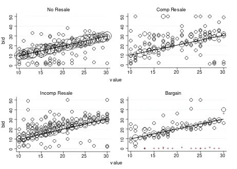
Figure 4.2: Strong Bidding – weighted scatterplot of observed bids (dropouts) by strong
bidders versus valuations in the four treatments.
With resale the strong bidder should reduce demand across all values, regardless of the form of the resale market or informational conditions.
Figure 4.2 plots weighted scatterplots of the observed strong bidders’ dropout bids against per unit value. We again include a line to show where a bid would be equal to value. In the no resale treatment (upper left graph of Figure 4.2) it is apparent that strong bidders dropped out at low prices with much higher frequency for values lower than 40. This is evidenced in two ways. First, we have larger clusters of zero bids for values below 40 and second, the number of observed bids is also much higher (showing that strong bidders dropped out …rst).
0 .2 .4 .6 .8 1
30 35 40 45 50 value No Resale 0 .2 .4 .6 .8 1
30 35 40 45 50 value Comp Resale 0 .2 .4 .6 .8 1
30 35 40 45 50 value Incomp Resale 0 .2 .4 .6 .8 1
30 35 40 45 50 value
[image:20.595.89.526.91.410.2]Bargain
Figure 4.3: Relative frequency of strong bidders winning both units, by strong bidders’ value, in the four treatments.
(p <0:001).27
To more accurately quantify the strong bidder’s response to both value location and the presence of resale, Figure 4.3 graphs the relative frequency of the strong bidder winning both units, broken down by value for all treatments. If a strong bidder reduced demand by dropping out of the auction …rst, he won 1 unit and the auction allocation was ine¢cient, otherwise he won both units in the auction. In the no resale treatment (…rst graph of Figure 4.3), strong bidders won 2 units more often when their value was higher than 40. A Kolmogorov-Smirnov (K-S) test indicates that the observed di¤erence between strong bidders winning when their
value was above 40 and below 40 is statistically signi…cant (p <0:001).
Turning to the resale treatments, it is immediately evident that the presence of resale
re-2 7For comparisons against the bargain treatment, both the full sample and restricted sample (20 periods per
sulted in much higher frequencies of demand reduction, although this e¤ect is lessened under incomplete information. We …nd signi…cant di¤erences between the no resale treatment and all
resale treatments for both high and low values (K-S, vS <40,p 0:007; vS > 40,p < 0:001).
Complete information resale and bargain appear most similar and we …nd no signi…cant
dif-ferences between these treatments (p = 0:264). Between incomplete information resale and
either complete information resale or bargain, signi…cant di¤erences exist whenvS was above 40
(p 0:001), but not whenvS was below 40 (p 0:102).
In theory, a strong bidder who reduces demand should drop out at zero. Yet any bid below 10, the lowest possible value of the weak bidder, can also be interpreted as strong demand reduction, since weak bidders should never drop out at a price lower than their value. Table 4.4 summarizes low-bidding behavior by strong bidders which is consistent with theory (conservatively de…ned as bids lower than 3). In the no resale treatment, 30% of all bids were near-zero dropouts when the strong bidder had a value less than 40. This percentage decreased substantially when the strong bidder had a value greater than 40. There is no comparable decrease in the resale treatments, but resale did result in the largest amount of near-zero bids, for both high and low values, particularly in the bargain treatment.
Percentage of Bids 2 No Resale Comp Resale Incomp Resale Bargain
vS<40 30% 37% 29% 48%
[image:21.595.106.495.361.407.2]vS>40 12% 40% 21% 41%
Table 4.4: Relative frequency of near-zero bids by strong bidders.
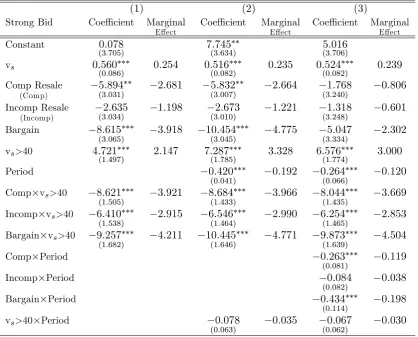
To examine strong bidders’ behavior in more depth, we analyze random e¤ects tobit models
in Table 4.5.28 Model 1 is our primary model of treatment and value location e¤ects. Models
2 and 3 explore learning e¤ects. The strong bidder’s unit valuation is represented by vS, while
vS >40 is a dummy variable indicating when the valuation was higher than 40. Comp Resale,
Incomp Resale, and Bargain identify treatment dummies, with the no resale case serving as the baseline. Period represents the period of play.
In the no resale treatment, the positive signi…cant coe¢cient onvS >40in Model 1 con…rms
that strong bidders’ bid higher when their values were above 40, implying less demand reduction when strong bidders had relatively high values. This provides empirical support for Result 1.
Empirical Result 3: Without resale, strong bidders reduce demand less with high value asym-metry between bidders — i.e., when vS >40.
Examining the e¤ects of resale, the signi…cant negative coe¢cients on Comp Resale, Bargain,
and the interactions of Comp Resale and Bargain withvS >40indicate that in these treatments
there was more demand reduction than without resale across all values, and especially for high
2 8All regressions include 1646 uncensored observations and 994 right-censored observations (at the auction
(1) (2) (3)
Strong Bid Coe¢cient Marginal
E¤ect
Coe¢cient Marginal
E¤ect
Coe¢cient Marginal
E¤ect
Constant 0:078
(3:705) 7(3:745:634) (35::016706)
vs 0:560
(0:086) 0:254 0:(0516:082) 0:235 0:(0524:082) 0:239 Comp Resale
(Comp)
5:894
(3:031) 2:681 5(3::832007) 2:664 (31::240)768 0:806 Incomp Resale
(Incomp)
2:635
(3:034)
1:198 2:673
(3:010)
1:221 1:318
(3:248)
0:601
Bargain 8:615
(3:065) 3:918 10(3::454045) 4:775 (35::334)047 2:302
vs>40 4:721
(1:497) 2:147 7:(1287:785) 3:328 6:(1576:774) 3:000
Period 0:420
(0:041) 0:192 0(0:264:066) 0:120
Comp vs>40 8:621
(1:505) 3:921 8(1:684:433) 3:966 8(1:044:435) 3:669
Incomp vs>40 6:410
(1:538) 2:915 6(1:546:464) 2:990 6(1:254:465) 2:853
Bargain vs>40 9:257
(1:682) 4:211 10(1::445646) 4:771 9(1:873:639) 4:504
Comp Period 0:263
(0:081) 0:119
Incomp Period 0:084
(0:082) 0:038
Bargain Period 0:434
(0:114) 0:198
vs>40 Period 0:078
(0:063)
0:035 0:067
(0:062)
[image:22.595.91.510.89.426.2]0:030
Table 4.5: Random e¤ects panel tobit - Strong bidding.
values. By contrast, the incomplete information resale treatment only resulted in signi…cantly more demand reduction than no resale for values greater than 40.
Empirical Result 4:With high value asymmetry between bidders, strong bidders reduce demand more with resale than without. With low value asymmetry between bidders, strong bidders reduce demand more with resale than without only in the bargain and complete information resale treatments. Demand reduction by strong bidders is highest in the bargain treatment.
4.3. E¢ciency and Seller’s Revenue
Auction e¢ciency is measured as the ratio between the valuation of the auction winner and the valuation of the strong bidder, which is the highest valuation. Since one unit was always awarded to the strong bidder, we will focus on the e¢ciency results for the second unit. Auction e¢ciency is lower than 1 when the weak bidder won the second unit because of demand reduction or speculation.
When an auction is followed by a resale opportunity, the e¢ciency generated by the auction allocation can potentially change. We refer to the post-resale e¢ciency as …nal e¢ciency, which is measured as the ratio between the valuation of the …nal holder of the good and the valuation of the strong bidder. In our environment, …nal e¢ciency is 1 if the weak bidder resold to the strong bidder after the auction; while …nal e¢ciency is equal to auction e¢ciency if no resale occurred. By Result 3 in Section 2, auction e¢ciency should be lower with resale than without, while …nal e¢ciency should always be 1 with resale, and higher than without resale.
Table 4.6 reports average e¢ciency, by treatment. No resale resulted in the highest auction e¢ciency, due to low levels of demand reduction by strong bidders with higher values. Yet, full e¢ciency is not reached without resale because strong bidders with lower values still re-duced demand. Pairwise WMW tests …nd signi…cant di¤erences in auction e¢ciency between
all treatments, except complete information resale and bargain (p= 0:519). Among the resale
treatments, incomplete information resale resulted in the highest auction e¢ciency.
Resale improved e¢ciency from the auction allocation to the …nal allocation, most strikingly when subjects were allowed to bargain or make take-it-or-leave it o¤ers with complete
infor-mation, consistent Result 3.29 Moreover, …nal e¢ciency in both the bargain and the complete
information resale treatments is higher than without resale. However, it is not necessarily the case that resale always yielded higher …nal e¢ciency: no signi…cant di¤erence exists between …nal
e¢ciency in the no resale and the incomplete information resale treatments (WMW,p= 0:103).
No Resale Comp Resale Incomp Resale Bargain
Auction E¢ciency 0:82
(0:241) (00::256)64 (00::258)71 (00::261)65
Final E¢ciency 0:82
[image:23.595.117.483.517.577.2](0:241) (00::170)93 (00::217)85 (00::132)95
Table 4.6: Average auction and …nal e¢ciency (standard deviations in parentheses).
Figure 4.4 examines e¢ciency through the relative frequency of the strong bidder holding 2 units after resale, depending on the strong bidders’ value. To show how the allocation changed after the auction, we have overlaid the auction allocation seen previously in …gure 4.3. Demand reduction in all resale treatments resulted in low e¢ciency after the auction, but resale increased …nal e¢ciency. With complete information or bargaining, the second unit was almost always
0 .2 .4 .6 .8 1
30 35 40 45 50 value final_relfreq intermediate_relfreq No Resale 0 .2 .4 .6 .8 1
30 35 40 45 50 value Final Auction Comp Resale 0 .2 .4 .6 .8 1
30 35 40 45 50 value Final allocation Incomp Resale 0 .2 .4 .6 .8 1
30 35 40 45 50 value
Auction allocation
[image:24.595.77.526.94.415.2]Bargain
Figure 4.4: Relative frequency of …nal allocation and auction allocation of 2 units to strong bidder, by strong bidders’ value.
transferred to the strong bidder when the weak bidder won it in the auction, and there is no statistically signi…cant di¤erence between the …nal allocations in these two treatments (K-S,
p = 0:485). Resale under take-it-or-leave-it o¤ers with incomplete information also increased
e¢ciency after the auction, but the …nal allocation for this treatment was similar to the no resale allocation. A K-S test con…rms that there is no signi…cant di¤erence between the allocation in the no resale treatment and the …nal allocation in the incomplete information resale treatment (p= 0:485).
Empirical Result 5: Auction e¢ciency is lower with resale than without. Final e¢ciency without resale is lower than in the bargain and complete information resale treatments, but is not signi…cantly di¤erent from the incomplete information resale treatment.
the auction winner. The highest overall revenue was achieved in the no resale treatment, but there is no signi…cant di¤erence between that revenue and the revenue in the incomplete
infor-mation resale treatment (WMW, p = 0:319). The reasoning behind the higher than expected
revenue with resale is straightforward: weak bidders bid more aggressively with resale, and this increased the seller’s revenue when strong bidders chose to win the auction rather than follow their equilibrium strategy and reduce demand. By contrast, consistent with Result 4, we do …nd signi…cant di¤erences between the revenue in the no resale treatment and the revenues in the
complete information resale treatment (p <0:001) and the bargain treatment (p <0:001).
No Resale Comp Resale Incomp Resale Bargain
Average Seller’s Revenue 14.61
(10.062) (12.448)11.94 (11.099)14.05 (10.567)8.47
Average Revenue - Weak Wins 8.01
(10.117) (11.339)8.64 (10.387)9.98 (8.873)5.25
Average Revenue - Strong Wins 18.81
[image:25.595.83.514.230.310.2](7.4 40) (10.181)21.85 (8.493)21.06 (9.849)17.22
Table 4.7: Average seller’s revenue per unit (standard deviations in parentheses).
Empirical Result 6: The seller’s revenue without resale is higher than in the complete in-formation resale and bargain treatments, but is not signi…cantly di¤erent from the incomplete information resale treatment.
Table 4.7 also shows that, in all treatments, the seller obtained a lower revenue when weak bidders won a unit, so that the auction price was determined by strong bidders’ bids (rather than weak bidders’ ones), although strong bidders had a higher willingness to pay per unit. This is consistent with the fact that strong bidders tended to reduce demand and bid lower than weak bidders, with intentions to reduce the auction price.
4.4. Resale Market
In this section, we highlight key aspects of the resale market that underlie the empirical regular-ities described previously for the resale treatments. Recall that the resale market either involved a take-it-or-leave-it o¤er where the proposer was determined with 50/50 probability (complete information and incomplete information resale), or placed bidders into an unstructured bargain-ing game (bargain).
Table 4.8 provides the relative frequency of resale in all resale treatments, and breaks this down into successful resale and failed resale. Successful resale took place when both participants agreed to an o¤er while failed resale was either a result of one of the participants choosing to exit
the resale stage or failed agreement before time expired.30 It is immediately evident that resale
3 0In the bargain treatment, we observed 72 cases of failed resale (out of 351 resale markets). Of these, 41 were
was more frequent and successful in the complete information resale and bargain treatments than in the incomplete information resale treatment; there is no signi…cant di¤erence between
the …rst two treatments in the frequencies of possible resale ( 2,p= 0:467) or success in resale
(p = 0:550). Incomplete information resale resulted in both a signi…cantly lower frequency of
possible resale (p < 0:001) and a signi…cantly higher rate of failed resale (p < 0:001). The
high occurrence of failed resale appears to depend on the mix of incomplete information and a take-it-or-leave-it o¤er mechanism.
Resale Possible
(weak won) Successful Resale Failed Resale
Comp Resale 75% 81:1% 18:9%
Incomp Resale 63:2% 42:2% 57:8%
[image:26.595.132.466.211.277.2]Bargain 73:1% 79:5% 20:5%
Table 4.8: Relative frequency of possible resale (when the weak bidder won a unit the auction), successful resale, and failed resale (out of Resale Possible).
From an e¢ciency standpoint, it is important to understand which factors determined a higher probability of successful resale in each resale mechanism. Table 4.9 provides marginal e¤ects from probit regressions with agreement to …nal resale as the dependent variable. Models 1 and 2 examine the complete and incomplete information resale treatments, respectively. The variable O¤er represents the take-it-or-leave-it o¤ers. Auction Price represents the dropout price
from the auction, Auction Price>vW is a dummy variable indicating when the auction price was
greater than the weak bidder’s value (i.e., losses at the auction stage for the weak bidder),
and vS vW represents the di¤erence between the strong and weak values to capture the e¤ect
of varying asymmetry between bidders. Weak Proposer is a dummy variable which indicates whether the proposer was the weak bidder.
The results indicate that, as expected, an increase in the o¤er made by a strong proposer signi…cantly increased the probability of …nal agreement by 2% in the complete information resale treatment and by almost 4% in the incomplete information resale treatment. Similarly, the interaction of o¤er with weak proposer is signi…cant and negative, showing that a reduction in the o¤er made by a weak proposer increased the probability of acceptance by a strong responder. We also …nd a signi…cant and large positive e¤ect of weak bidders assigned to the proposer role on the probability of agreement, arguably because weak bidders were less aggressive in the resale market than strong bidders, as shown below.
Although in theory the pro…ts from the auction should not a¤ect the resale market, in the incomplete information treatment we …nd a strong positive e¤ect when the auction price was higher than the weak bidder’s value. Speci…cally, if the weak bidder paid an auction price higher than his value, incurring losses at the auction stage, the probability of resale agreement increased
by 13%. The size of the gains from tradevS vW had little impact under complete information,
(1) (2) (3)
Final Resale Agreement Comp Resale Incomp Resale Bargain
O¤er 0:019
(0:005) 0:(0037:013)
Initial Weak O¤er – Initial Strong O¤er 0:011
(0:0005)
Auction Price 0:003
(0:003) (00::001)0003 0(0:0001:002)
Auction Price>vw 0:060
(0:082) 0(0:134:067) (00::036101)
vs–vw 0:004
(0:004) 0:(0022:006) 0:(0011:001)
Weak Proposer 0:651
(0:037) 0:(0705:193)
O¤er Weak Proposer 0:021
(0:005)
0:032
(0:015)
Auction Price Weak Proposer 0:003
(0:002) (00:001):003
# O¤ers Made 0:009
(0:005)
Observations 534 445 344
[image:27.595.105.494.89.339.2]Clusters 3 3 3
Table 4.9: Marginal e¤ects from Probit regressions on resale of unit (…nal resale agreement), conditional on weak winning. Standard errors clustered at the session level.
likely because it increased the range of potential o¤ers that led to positive pro…t in the resale market for both participants.
Turning to the bargain treatment in Model 3, we restructured the estimated model to account for the di¤erent resale mechanism. Because of the unstructured process of the bargain treatment, we typically observe a series of alternating o¤ers rather than a single o¤er. To determine the role of o¤ers under bargaining, we take the …rst o¤er made by both strong and weak bidders, and di¤erence these. If agreement was reached with a single initial o¤er, this di¤erence is de…ned as zero. We also include a variable, # O¤ers Made, which tracks the total number of o¤ers made by a bargaining pair. We …nd that the distance between the weak and strong initial o¤ers negatively impacted the probability of …nal agreement: every 1 unit increase in distance implied a 1.1% decrease in the probability of acceptance. We also …nd a signi…cant, but relatively weak negative e¤ect for the number of o¤ers made. As in the incomplete information resale treatment, higher value asymmetry increased the probability of successful resale.
Empirical Result 7:Resale is more likely to succeed when the weak bidder has more bargaining power, with more information in the resale market, larger gains from trade, and ‡exibility in the bargaining mechanism. Bidders trade most often (when it is e¢cient to do so) in the bargain and complete information resale treatments.
signi…cantly higher in complete information resale than either bargain (WMW, p < 0:001) or
incomplete information resale (p <0:001). For bargain and incomplete information resale, the
di¤erence is not signi…cant (p= 0:437). There are also signi…cant di¤erences in earnings between
strong and weak bidders in all treatments, but the relationship is statistically weaker for the
complete information resale treatment (p = 0:065) than the incomplete information resale and
bargain treatments (p <0:001). Hence, weak bidders obtained a lower pro…t than strong bidders
in the resale market, but managed to obtain relatively higher pro…ts with complete information
where pro…ts were closer to equal splits of the resale surplus.31 Di¤erences in earnings were
mainly driven by strong bidders making more aggressive o¤ers in the resale market, especially with incomplete information. Contrasting the o¤ers for the take-it-or-leave-it treatments, strong
proposers made signi…cantly lower o¤ers under incomplete information (p < 0:001), while we
…nd no signi…cant di¤erences between o¤ers made by the weak proposers (WMW,p= 0:345).
Resale Price Weak Earnings Strong Earnings Resale O¤er
Weak / Strong
Comp Resale 29.56
(5.619) (5.527)9.45 (5.749)10.20 (4.664)32.47=(6.240)25.45
Incomp Resale 27.38
(7.686) (7.964)8.74 (7.635)12.59 (6.911)32.45=(7.035)17.93
Bargain 27.44
(4.474) (5.866)8.35 (6.559)12.43
-Table 4.10: Average resale prices, resale earnings, and o¤ers by type (standard deviations in parentheses).
Comparing average resale prices from Table 4.10 to average auction prices (which are equiv-alent to the seller’s revenue) from Table 4.7 it is clear that, in all treatments with resale, on average, auction prices are lower than resale prices. This di¤erence is particularly large in auc-tions where the weak bidder wins and there is pronounced demand reduction by strong bidders; but resale prices are also higher than auction prices even when the strong bidder wins and the auction is not followed by a resale market. Signed rank sum tests by treatment con…rm
signi…cant di¤erences between the auction and resale prices for all resale treatments (p <0:001).
Finally, Table 4.11 reports total bidders’ pro…ts — i.e., auction earnings plus resale earnings — by types and treatments. As these earnings are cumulative, for comparisons to the bargain treatment we restrict all treatments to 20 periods of data. Pairwise WMW tests …nd signi…cant
earnings di¤erences for both weak (p < 0:001) and strong bidders (p 0:003) across all
treat-ments. Weak bidders obtain higher pro…ts when resale is allowed, because of the option value of selling the units acquired after the auction. By contrast, strong bidders obtain higher pro…ts when resale is allowed only when the resale market is su¢ciently e¢cient, so that they manage to trade with high probability after the auction.
3 1In the resale treatments with take-it-or-leave-it o¤ers, the bidder who is chosen as the proposer should make
[image:28.595.100.499.299.383.2]