Adaptive Filter for High Dimensional Inverse Engineering Problems: From Theory to Practical Implementation

Adaptive Filter for High Dimensional Inverse Engineering

Problems: From Theory to Practical Implementation

Hong Son Hoang, Rémy Barailles

HOM, SHOM, Toulouse, France Email: [email protected], [email protected]

Received February 22, 2013; revised March 23, 2013; accepted April 1,2013

Copyright © 2013 Hong Son Hoang, Rémy Barailles. This is an open access article distributed under the Creative Commons Attribu-tion License, which permits unrestricted use, distribuAttribu-tion, and reproducAttribu-tion in any medium, provided the original work is properly cited.

ABSTRACT

The inverse engineering problems approach is a discipline that is growing very rapidly. The inverse problems we consider here concern the way to determine the state and/or parameters of the physical system of interest using observed measurements. In this context the filtering algorithms constitute a key tool to offer improvements of our knowledge on the system state, its forecast… which are essential, in particular, for oceanographic and meteorologic operational systems. The objective of this paper is to give an overview on how one can design a simple, no time-consuming Reduced-Order Adaptive Filter (ROAF) to solve the inverse engineering problems with high forecasting performance in very high dimensional environment.

Keywords: Dynamical Systems; Adaptive Filtering; Stability; Real Schur Decomposition; Stochastic Approximation; Numerical Prediction; Data Assimilation

1. Introduction

Filtering algorithm constitutes a key tool to offer im- provements of system forecast in engineering systems, in particular for oceanographic and meteorologic operational systems. Theoretically, the optimal filtering algorithms provide the best estimate for the system state based on all available observations. As many engineering problems are expressed mathematically by means of a set of partial differential equations together with initial and/or bound- ary conditions, their numerical solutions result on system state with very high dimension (order of ). In this context the adaptive filter (AF) for state and para- meter estimation is an attractive topic for the last decades [1]. Traditionally, the AF is a filter that self-adjusts its parameters (of transfer function) to minimize an error signal. The corresponding nonadaptive filter has then a structure obtained by conventional methods. The AF uses feedback in the form of an error signal to adjust its tuning parameters to optimize the filter performance. It offers an attractive solution to filtering problems in an environ- ment of unknown statistics, provides a significant im- provement in performance. AF is successfully applied in many fields as communications, control, noise cancella- tion, signal prediction, radar, sonar, seismology, biome- dical engineering...

6

10 -107

7

One other potential field of application of the AF is numerical weather prediction, in particular, data assimi- lation. It uses mathematical models of the atmosphere and ocean to predict the weather based on current esti- mates of weather state [2]. With vast data sets and di- mensions of the system state of order , data as- similation requires the most powerful supercomputers in the world. Even though, at the present, for operational purposes we must be satisfied with simplified assimi- lation methods, not to say on implementation of sophi- sticated forecast optimal techniques like a Kalman filter (KF) [3] in near future due to requirement on huge me- mory storage and time evolving the system of equations of dimension The difficulties encountered here concern not simply very high dimension of the sys- tem state. Factors affecting the accuracy of numerical predictions include the uncertainty in model error sta- tistics, a more fundamental problem lying in the chaotic nature of the partial differential equations used, the den- sity and quality of observations... These difficulties re- quire an another approach to the design of assimilation systems for improving the performance of weather fore- casting skills. The objective of this paper is to give an overview of how one can design a simple, no time-con- suming Reduced-Order AF (ROAF) with high forecast-

6

10 -10

12 14

ing performance to handle assimilation problems in the very high dimensional environment.

In the section that follows a brief outline of the theory of ROAF is given. The steps in implementation of the ROAF are detailed in Section 3. Numerical experiments are formulated in Sections 4 and 5 where the problems of estimation of the trajectory of the Lorenz system as well as assimilation of sea surface height (SSH) into the oceanic model are exhibited. Section 6 includes the con- clusions.

2. Theoretical Aspects

2.1. Why the Adaptive Filter

The AF, in the context of that designed for estimating the state of very high dimensional system, originates from the work [4] which is defined as a filter minimizing the mean prediction error (MPE) of the system output. One of the main features of the AF is that it is optimal among the members of a set of parametrized state-space inno- vation representations, with the vector of pertinent para- meters of the gain as a control vector. Consider the stan- dard filtering problem



1



 

 

,

x k F x k_ _w k k1, 2,.

1, 2,

(1)



1



   

,

z k Hx k v k k . (2) here _{x k}

 

_{R F}n,

 

 :_Rn_{R H R}n, : n_Rp,_{w k}

   

,_{v k}

Q R

are uncorrelated sequences of zero mean and time- invariant covariance and respectively. For sim- plicity, in (2)

 

 

F x k_ _ x k (3) The optimal in mean squared filter is given then by the KF,





 

   

 

ˆ 1 ˆ ˆ

1, 2,

,

x k x k K k z k H x k k

    _   _

  (4a)

 

 

_T

 

_T 1 ,

K k M k H _HM k H R

,

(4b)





 

T

1

M k  P k  Q

T

(4c)

























T T

T

1

1 1 1

1 1 .

P k

I K k H M k I K k H K k RK k



  

_   _  _  

  

6 7

(4d)

For systems with a dimension of order un- der most favorable conditions (perfect knowledge of all system parameters and noise statistics...) it is impossible to implement the filter (4) in the most powerful computer systems in the world.

10 -10 ,

In order to exploit the optimal structure of the filter

like (4a), noticing that in (4a) all the variables are well defined except the gain K k

 

. Moreover, under mild conditions, the gain K k

 

will converge to a constant

 

K  [3].

Thus if instead of all equations in (4) we use only the first equation with assumption that K k

 

K, K is constant, there is an expectation that one can design a filter which is close to the optimal one if K is close to

 

.

K  However such asymptotically optimal filter is realizable only if the system dimension is relatively small. To be able to work with any system independently of its dimensionality, in [4] the filter is assumed to be of the form (4) with the gain K:K

 

 well defined up to the vector of unknown parameters . Then instead of finding all elements of K, the task is reduced to seeking an optimal  of dimension n_, which, as expected, is much less than The best way to carry out this task is to introduce the MPE objective function [4]

.

n

 



 



min

J  E  k   (5a)

 





 

 

  



2 ,

ˆ

: 1

k k

k z k z k k

 



 

   (5b)

where E

 

 is the mathematical expectation operator,

 denotes the l2 vector norm, z k kˆ



1



represents a one-step-ahead predictor for Mention that the gain in the KF minimizes the objective functions (5a) and (5b) too (under the condition on perfect knowledge of all noise statistics and system parameters...) since

 

.

z k



1



ˆ

z k k represents the innovation vector.

Introduction of (5) gives us a great advantage in the design of an ROAF since its minimization can be per- formed by a simple stochastic approximation (SA) al- gorithm [5]: At each assimilation instant one has to com- pute only the gradient of the sample objective function

 



 k



 . This makes the task filter design much simp- ler compared to the KF where the estimation error is minimized in the probability space hence requires the knowledge of probability density functions of all entering random variables. As to Four-Dimensional Variational (4D-Var) [6], the optimization is performed over all as- similation period by iterative algorithms which require, at each assimilation instant, about 20 iterations (each iteration includes one forward model integration and one backward adjoint integration) to approach an optimal control vector. The principal differences between two ap- proaches, 4D-Var and AF, are listed in Table 1.

2.2. Order Reduction and Gain Parameterization

2.2.1. Order Reduction

[image:3.595.59.287.100.203.2]

Table 1. Main differences between 4D-Var and AF.

Approach 4D-Var AF

Control vector Initial system state Gain parameters

Objective function

Misfit between output

and observations MPE of system output

Optimization Batch-vector, iterative SA, Sequential

Gradient computation

Integration of model and adjoint equations over

assimilation period

Integration of model at each assimilation instant

the gain,





 





ˆ 1 ˆ 1 , : _{r e}

x k  x k K k K PK



(6)

where projects correction from the

reduced space into the full space, e



e nxn

r e

PR n n

K represents the gain in the reduced space. In [7,8] the choice of rand

parameterization of the gain e

P K are studied from the point of view of filter stability. It is well known whatever is a filter, the question of ensuring its stability is of the first importance: instability causes the error growth and it can completely destroy the filter. It turns out that under detectability condition, stability of the filter can be gua- ranteed if the columns of r is constructed from a sub-

space of unstable and neutral eigenvectors (EVs) or sin- gular vectors (SVs) of . From a computational point of view, it is inadvisable to construct r from leading

eigenvectors or singular vectors: the eigenvectors may be complex, non-orthogonal hence their computation suffers from numerical instability. A great advantage of the sin- gular vector approach is that it does not suffer from nu- merical instability. There exists the efficient Lanczos al- gorithm [9] for computing the leading singular vectors of very large sparse systems. However, definition of singu- lar vectors depends on an introduced vector norm and their computation requires the adjoint of

P



P

T _

. For many physical problems, the latter represents a very hard task, not to say about the possible existence of discon- tinuities when obtaining the tangent linear model (TLM)

.



The third approach is related to leading (or dominant) real Schur vectors (ScVs). As proved in [7], the real dominant ScVs (DScVs) play the same role in ensuring filter stability as the dominant EVs or SVs. The Schur approach enjoys all advantages of the singular vector ap- proach and in addition, it does not require the adjoint code. Computation of DScVs is closely associated with searching the direction of rapid growth of the prediction errors (PE). In [10] the PE sampling procedure (SP) based on DScVs is proposed which is aimed at gene- rating the PE samples for the DScVs. These PE samples (will be referred to as DPE (dominant PE) samples) will participate in the construction of r or in the estimation

of the parameters of to initialize the gain.

P

K

2.2.2. Gain Parametrization

In [7] different structures of Ke are proposed which

ensure a stability of the filter (6) if r is constructed

from either dominant EVs or DScVs. For

P

1

T T

, :

e e e e e e e r,

K M H _H M H R_ H HP (7)

the symmetric positive definiteness (SPD) of Me can

guarantee a stability (in norm) of the filter. Thus parameterization of e

2

l

e

M M

 

 can be made with  as a vector of tuning parameters provided that Me

 



should be SPD. For adaptation purpose, the following stabilizing gain structure is of more interest due to linear dependence of the gain on the tuning parameters



1

, diag , , _e , 0, 2

r e n l

K P K   _  _  



(8)

2.3. Numerical Approximation of P r

Generated PE samples share the important property to be iteratively developed in directions of rapid growth of the prediction error. The columns of constructed from DScVs, allow for capturing the most growing PEs. In [10] the PE sampling procedure is proposed for generating the DScVs samples:

,

r

P

Consider the system (1) at the moment and let ti

 

f

x i —some estimate for the true system state x i

 

— be given. The estimation error is x i

 

xf

   

i

 

 i x . Integration of the model from xf i produces the pre-

diction x_p



i  1



x_f

 

i at ti1 ti t. Here

 

f x i



t

represents model integration over the interval

 . As the true system state at ti1 is x i



 1



x

 

i (for no model error case), the PE



1



 

 

p f

e i  x i  x i  x i

 

. Thus integrating

 

x i

 by the model yields the vector si1 x i

 

which can be considered as a PE pattern growing over the period of model integration t. If we apply this procedure to an ensemble of orthogonal columns

 

 

1

, , L

i

X  x i  x i _ instead of one vector x i

 

, the iteration S_i X X G_i, _{i i}S i_i, 1, 2,will produce the sequence

 

Xi approaching dominant Schur

vectors of

L

 . The operator r thus can be appro-

ximated by using the columns-vectors of i which be-

long to the subspace generated by columns of i

P

S

X . The filter with the gain constructed on the basis of PE sam- ples will be referred to as a PE filter (PEF).

2.4. Optimization

the AF can improve its performance that the traditional filters cannot. The objective (5) is based on the deep philosophical idea postulating that the best model should be able to predict the future real process with high pre- cision. As uncertainty in the model always exists, even the KF cannot produce the best estimation in such situ- ation.

From the computational point of view, the choice of the criteria (5) allows us to greatly simplify the opti- mization procedure. Since the optimality is understood in the mean probabilistic sense, simple optimization tools known as stochastic approximation (SA), and in parti- cular, a simultaneous perturbation SA (SPSA) [5], are quite appropriate for seeking the optimal parameters. With the SPSA, one can compute the gradient vector by additional two times integrating the numerical model. The algorithm is independently on dimension of the vec- tor of tuning parameters. Thus no adjoint equation (AE) for is needed for the optimization procedure whose construction is a hard task, not to say on the com- putational time and the cost of integrating AE, possible existence of discontinuities in the numerical model, of non-linearities... For more details, see [11].

T

 

3. Practical Implementation of ROAF

The following steps are to be proceeded in order to con- struct a ROAF.

Step 1. Simulation of an ensemble of DPE samples: (i) Choice L—a number of DScVs;

(ii) Apply the Sampling Procedure (SP) in [10] to generate an ensemble of PE samples

for L DScVs.

 

, 1, 2, ,

i

S L i  T

Step 2. Estimation of the filter gain: (i) Choice of gain structure;

(ii) Estimation of the gain elements from generated PE samples S L i_i

 

, 1,,T;

(iii) Parametrization of the gain with  as a vector of unknown parameters.

Step 3. Optimization of filter performance: Apply the SPSA algorithm to estimate the tuning parameters . This algorithm is of the form (see [5])



k 1



 

k kg



 

k



,

     (9a)

 







 





 



T

1

: , , n

g  k  g  k  g_  k _ ,



(9b)

 





 



;





;

 

, 2

i

k k k k

k k

g k

k c k c

c



   

      





(9c)

where   k



k1,,kn



T,kican be chosen as ran-

dom variable having the symmetric Bernoulli (+/–) 1 distribution.

For sufficient conditions for convergence of the SPSA iterate 

 

k , see [5]. In [11] a comparative study on the efficiency of the SPSA with respect to other stan- dard optimization methods shows that the SPSA is more efficient when it is applied to optimizing nonlinear sys- tems and/or when more and more observations are assi- milated (the experiment on estimation of the vehicle’s present position and velocity).

Comment 3.1. Due to orthognormalization X Gi iSi,

the columns of Xi are normalized, as a consequence

the columns of Si1 Xi represent only the direction

but not the amplitude of PE. For the renormalization pro- cedure, see Comment 2.1 in [10].

Comment 3.2. If at i1 one assigns



1







x_f i x_p i1 , the SP generates PE samples using only the numerical model. We have then a so called off- line SP (denoted as SP1). In the so-called on-line SP (SP2) the samples are generated during the filtering process. The SP2 simulates the PE by integrating the mo- del from the filtered and its perturbed estimate. The re- normalization process can be performed then more pre- cisely if there is a possibility to get some information on the ECM matrix P k

 

of the filtered error ef

 

k at

: _k

k t assimilation instant (see (4)). For 1 -square-

root of



P k



   

   

T

1 P1 k

,

P k P k P k , the filtered error (FE) sample is obtained from the relation

 

1

 

 

, 1, 2, , .

l l

f p

x k P k x

   k l  L The PE patterns in

SP2 are generated by integrating the model from

 

ˆ

x k and ˆ

 

l

 

f

x k x k at each assimilation instant. They can be used to correct the ECM obtained by the off-line SP1 and to improve the filter performance.

Comment 3.3. For the systems with moderate state dimensions (see the Lorenz system in Section 4), all the elements of the matrix M:M k

 

 

, 1

i

S L i

in (4) can be esti- mated from the ensemble , for example, by

,,T

1

1 ˆ ˆ : ,

T i i

M M M B T 

 



(10a)

 

 

 

 

T ,

1 1

1

,

L

l l T

i i i p p

l

l l

p p

B S S i i

L i x i

 

 



  

 



(10b)

where    1 1T represents a re-normalization factor.

For very high dimensional systems, the matrix Me ob-

tained from (10a) is rank deficient. It is therefore advi- sable to select a well defined structure of the gain with a small number of parameters to be estimated from PE samples. See Section 5 for more details.

complex, non-repeating pattern [12].

4.1. Problem Statement

The equations that govern the Lorenz attractor are:



1

1 2

d

, d

x

_

x x

t    (11a)

2

1 2 1 3

d

, d

x

x x x x

t    (11b)

3

1 2 3

d

, d

x

x x x

t   (11c)

where  is called the Prandtl number and  is called the Rayleigh number. All   , , 0, but usually

10, 8 3

   and  is varied. The system exhibits chaotic behavior for 28 but displays knotted pe- riodic orbits for other values of  . In the experiments to follow (see also [13]) the parameters   , , are cho- sen to have the values 10, 28 and 8 3 for which the “butterfly” attractor exists.

It is assumed that the observations arrive at the mo-

ments 1 The system

(11) is discretized using the Euler method, with the model time step 1

, 1, 1, ,100.

k k k k

T T_ T   T k 

, 0.005

i i

t t t t

  _   

 

. Thus the obser- vations are available after each 200 steps of model in- tegration. The dynamical system corresponding to the transition of the states between two time instants kand

1

k thus can be represented in the form (1) with non-

linear

T T_

F  . In (1) w k

 

simulates the model error. The sequence w k

 

is assumed to be a white noise having variance 2, 12.13 and 12.13 respectively. As to the observation system, the operator



_{T T}



T







1, 2 , 1 1, 0, 0 , 2 0, 0,1

H h h h  h 



, i.e. the first and third components x x1, 3

0.

are observed at each time ins- tant T kk, 1,,10 The noise sequence v k

 

is white

with zero mean and variance R2I2 where Inis unit

matrix of dimension The initial estimate in all filters is given by

The true system state .

n

  

0 1.508 91 .



T

 

ˆ

x  870, 1.5312 71, 25.460

x k







ˆ 0

x

is modeled as the solution of (1) (2) subject to added by the Gaussian noise with zero mean and variance 2. The problem considered in this experiment is to apply the PEF and EnKF for estimating the true system state using the observations

and to compare their performances (see [10] for details).

 

,k1, 2,

z k

4.2. The EnKF, PEF and Assimilation

The SP1 has been applied to generate the ensemble of patterns S L_i

 

:_xl_p

 

i i, 1,,L_. The pattern

 

l p

x i

 is obtained at Ti,  Ti Ti1 Ti 1, i.e. over

the interval equal to that between two observation arrival

times. After T iterations, the ECM M is estimated using Equations (10a) and (10b) on the basis of



,





_i

 

, 1,



S L T S i T

,

L

: k.

k T

L

 , . The gain of the PEF is

computed according to the equation for K in (4) subject to the obtained time-invariant M (for a fixed T). Accord- ing to [14], the gain in the EnKF is updated using the associated Riccati equation and an ensemble of pertur- bations of the size at each assimilation instant



Evolution of the gain element (2,1) in the EnKF sub- ject to L100 is shown in Figure 1. Mention that for

L = 3, L = 30 (not shown here) the variations of the gain in the EnKF are much stronger than for . It hap- pens since the perturbations in the EnKF are of random characters. The variation becomes less important with increase in the ensemble size. As reported in [15], the EnKF can yield an accurate performance if the ECM is estimated on the basis of the ensemble of 1000 samples.

100

L

The corresponding gain element in the PEF is shown in Figure 1 too. The curves PEF-L1, PEF-L2, PEF-L3 correspond to three simulations subject to L1, 2, 3 respectively. They are sufficiently smooth after about 20 iterations and behave in a similar way. Generally speak- ing, the gain element (2,1) in the PEF is greater than that in the EnKF.

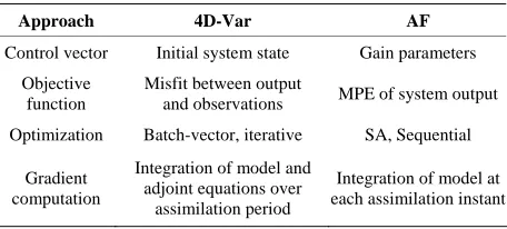
Time-average Root-Mean Squrare (RMS) of the FE (RMS-FE), resulting in two filters EnKF and PEF subject to different gains, are presented in Figure 2. In the PEF the gains are time-invariant assuming the values at

100

[image:5.595.324.519.553.720.2]

T  (see Figure 1). At the end of the assimilation process, with exception of the EnKF-3, all the filters yield almost the same error level. The RMS of the PE (RMS-PE) produced by the EnKF-3 is too high



RMS10.4



, i.e. being 1.42 times higher than that of the PEF-L1 (with RMS7.3). It is important to stress that due to very slow convergence rate in the Monte- Carlo method, the performance of the EnKF can be im- proved only at an expensive computational cost since the

[image:6.595.75.268.85.253.2]

Figure 2. RMS-FE in EnKF and PEF. ensembles of very large size must be simulated.

In the Lorenz system, for the PEF, the maximal en- semble size (at each time instant) is equal to the dimen- sion of the system state, i.e. equal to 3. Implementation of the EnKF-30 requires, at each assimilation instant, 30 times integration of the numerical model. That is 10 times greater than the dimension of model state. As reported in [15], the EnKF with 19 ensembles produces the estima- tion error of 3 times higher than that based on 1000 en- sembles. In contrast, even with , the performance of the PEF is comparable with that of the EnKF-100.

1

L

5. Assimilation in Oceanic Model

5.1. Numerical Model

In this section the ROAF is constructed and applied to assimilate the Sea Surface Height (or topography or re- lief of the ocean’s surface). The ocean model used here is the Miami Isopycnal Coordinate Ocean Model (MICOM). For the detailed description of the model, see [16]. The model configuration is a domain situated in the North Atlantic from 30.0 N to 60.0 N and 80.0 W to 44.0 W. The grid spacing is about in longitude and in lati- tude, requiring Nh = Nx × Ny = 25200 (Nx= 140, Ny = 180)

horizontal grid points. The number of layers in the model is We note that the state of the model is

0.20

4.

z

N 



, ,



x h u v

1,11, ,

where is the thickness of the

lr-th layer, are two merid-

ional and zonal velocity components. The state of the model has the dimension In the twin ex- periments to follow it is assumed that we are given the noise-free observations each (days) not at all grid points at the surface but only at the points



i j l, , ,v v n

10 ,171.





hh r



, ,j lr



i,



302

ds ,11,

 



,

u u i  j lr

, 400.

31; 1

i 1 j

5.2. SSH Observations: Reduced-Order Filter

The assimilation problem can be formulated in the form

(1) (2) where x k

 

 _h k u k

     

, ,v k _ is the system state at k:t tk,k1 tk 10 ds, F

 

 represents the inte-

gration of the nonlinear model over 10 , is the filter gain,

ds K

 

k



.

oi

is the innovation vector. The gain has the structure 1

K

KK P The operator oi will in-

terpolate the missing observations from observed points to all horizontal grid points. Symbolically

P

1

K is given

by



T T



1 , u, v

T

h

K  I K K K where K Ku, v are the opera-

tors producing correction



 u, v





h oi

for velocity from layer thickness correction K P k



using the geo- strophy hypothesis. This gain structure can be obtained also by assuming that the covariance M has the verti-cal and horizontal separable structure. By considering

 

oi

P z k instead of z k

 

, the observation operator can be regarded as H  Ip,,Ip where Ip is the

unit matrix of dimension



pxp



( is the number of all horizontal grid points).

h

pN

5.3. Structure of ECM and Its Estimation

As mentioned in Comment 3.3 (Section 3), the formulas in (10a) and (10b) are appropriate for estimating all the elements of the ECM M k

 

only if the system has a moderate dimension (see the Lorenz system in the pre- vious sections). For very high dimensional systems, in- stead of (10a) and (10b) we introduce the structure



1



_e, _p

M    M     I (12a)

 

, _{, 1}, 0,1

z N l m _{l m}

 



  

 _{ }  (12b)

where  denotes the Kronecker product; Nzis the

number of thickness layers in the model, l m, is a scalar representing the covariance of the PE between two layers

and The elements l m,

l m.  can be chosen a priori

from physical considerations or estimated from PE pat- terns. In the well-known Cooper-Haines filter (CHF, see [16,17]), the elements l m, are deduced from several physical constraints (conservation of potential vorticity, no motion at the bottom layer...). In the PEF, l m, are estimated from DPE patterns. Applying the SP1 subject to L1 yields the ensemble of DPE patterns



, ,j lr k;



,k1,,

p from which l m,

h i T

  can be esti-

mated through







, , ,

1

1 , 1

, , ; , , ;

T

k k l m l m l m

k T

p p

ij

T

h i j l k h i j m k p

  

 













(13)

where span all horizontal grid points whose number is equal to As the ensemble

,

i j

.

p



, ,j lr;k



, 1, ,

p

h i k T

alone, for fixed T, the matrix  is constant.

In what follows we reserve the notation PEF for the filter subject to ECM (12) with  0.

T

For 2 _,

r p

R I

1 substituting (13) into KMH _HMHTR

 

 (see the gain in (4)) leads to

 

T

, 1

, '

z

z

f N m N m m

2 , 1

1 , , ,

,

, 2, ,

pe p

l m l

m m r, 1 z h

K k k N I

k

s

s l N



  

 



  













 

 

.

For the present MICOM model, , the gain in the CHF [2] is equal to

2

0

r

 



18 .965



.

chf 5.965, 0, 0,184 p

K  I

5.4. Parametrization of the Gain. Adaptive Filter

Let estimated from (13), be decomposed as Subject to (6), the gain

,



DDT.

  K_pef is represented

as Kpef  P Kr e,PrD where



1 4



diag ,, I_p,_l 0

  with Ke defined as in

(7). The adaptive PEF (APEF) is obtained by adjusting , 1, , 4

l l

  

 

0 1, 1 4

l l

  

R

to minimize (5). The initial values

correspond to the non-adaptive PEF. For noisy-free observations, we have

,,

22.14

0,



62.54

 





T

120 2 , 81.38, , 77.21 .

pef p

[image:7.595.334.513.84.225.2]

K     I

Figure 3 shows the gain coefficient in the PEF obtained as functions of iteration resulting during application of SP1. Here

 

3

k i

,

l m

 are estimated in accordance with (13) during application of SP1 subject to L1 (curve “1L”) and (curve “5L”). It is seen that the estimation procedure is robust to the size of sample ensemble.

5



L



L

5.5. Performances of CHF, PEF and APEF

Figure 4 shows the time evolution of the sample ob- jective function (variances of the SSH inno- vation) resulting from CHF and PEF.

 

k



 

It is seen that the patterns generated by SP1 allow to well estimate the gain coefficients and as consequence, to improve significantly the performance of PEF compared to that of the CHF: in average, the reduction is of order 50% for the SSH-PE. As to the velocity estimation error, the reduction is of order 40% [11].

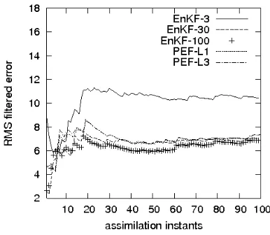
The algorithm SPSA (9a)-(9c) has been applied to mi- nimize the objective function (5). Figure 5 shows how the gain component k

 

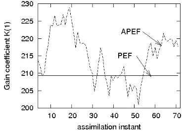
1 in the adaptive PEF (APEF) varies during adaptation whereas the gain in the PEF is constant. As expected, self-adjusting the gain parameters allows the APEF to reduce significantly the estimation error that the PEF cannot (see Figure 6).

[image:7.595.330.513.86.395.2]

-25

Figure 3. Estimated gain coefficient k 3

 

.

Figure 4. Variances of SSH innovation in CHF and PEF.

Figure 5. Gain in PEF and APEF.

5.6. On-Line SP2

In order to search other opportunities to reduce the es- timation errors, the SP2 has been applied along with a re-normalization procedure, without or with the use of Riccati like equation (see Comment 3.2). This allows us to utilize the PE samples generated during assimilation. First we assume that

 

 

  



0

 

,

1 .

p

M k M k I

M k  k



 

     

[image:7.595.330.514.426.559.2]

[image:8.595.75.272.85.228.2]

Figure 6. Sample cost functions in PEF and APEF. ated

r by SP1 and 

 

k : 

 

k Ip is estimated from

[image:8.595.327.515.85.217.2]

patterns generated by ilation.

Figure 7 shows SSH PE variances produced by the PEF subject to 0

SP2 during assim

 (denoted as PEF0) and 0.3 (PEF03). Thus by using PE samples, generated during assimilation, it is possible to extract in addition the information on the prediction error and to obtain a more precise PE covariance matrix and hence to improve the filter performance.

Another way is based on employing a Riccati like equation to estimate the filtered error (FE) patterns. Once having 

 

k , the ECM of the FE is estimated using the Riccati like equation

 

 

 

 

 

 

 

 

T

T

, ,

L L

N N

p p p

I K k H k I K k H

K k R K k P k

K k K k I H H I R R I

      

_  _ _ 

  



 

     







Decomposing and following

Co

 

   

T

1 1

P k P k P k

can re-normalize

mment 3.2 one xlp

 

k as

 

: 1

 

 

.

l

f p

 l

x k P k x k

   The ense e o PE samples

l l

mbl f



1



ˆ

 

_f

 

ˆ

 

p

x k F x k x k   _ F x k_ _ is generated

 _

at the next k1instant and the new

l p



k1



is esti-

 

mated from x



k1 ,



l1,, .L

In Figure 8 -RIC” repres e SSH

PE error pro s



the curve “PEF ents th

duced by the PEF who e gain is updated on the basis of L10PE samples simulated at each assi- milation instant. It is clear that the “PEF-RIC” behaves better than the “PEF”, especially as assimilation pro- gresses. The price to pay here (compared to PEF) is that one needs to integrate in addition L times the numerical model at each assimilation instant k.

6. Summary

Theory and practical implementation of the ROAF are presented in this paper. This offers a unified approach to the design of an efficient ROAF with low computational

Figure 7. Performance of PEF subject to 0 and .

0 3

 (see (12)).

Figure 8. PEF with the gain updated during assimilation by Riccati like equation.

cost. It is developed to overcome e difficulties encountered in the filtering problems with

efficient w

and computer memory th

very high dimensionality of the system state, uncer- tainties in the system description, non-linearities... The purpose of this paper is not only to give a comprehensive understanding the basic ideas behind this theory but also intended to provide the potential practitioners a guide for implementation of the ROAF. The ROAF design essen- tially consists of: 1) Choice of filter gain; 2) Application of a rather simple, but quite powerful PE sampling proce- dure for generating the PE samples which will participate in the construction of projection subspace and/or initiali- zation of the filter gain; 3) Parametrization of the filter gain and optimization of filter performance by imple- menting an efficient and low-cost SPSA algorithm which allows to evaluate the gradient of the objective function by 2 times integration of the numerical model.

We mention that compared with traditional optimi- zation methods, the SPSA is proved to be more

[image:8.595.344.503.261.384.2]

e PE

[1] S. Haykin, “A tice Hall, Up-

per Saddle Riv

ography,” Advances in Geophy-dimensional systems) the innovation 

 

k does not form an uncorrelated random process and one natural way to improve the filter performance is lude a pro- cedure for whitening the sequence 

 

k . This task can be done efficiently by assuming 

 

k to be a solution of a Markov equation, along with tunin nown parame- ters to minimize the variance of th system output.

REFERENCES

to inc

unk g

daptive Filter Theory,” Pren er, 2002.

[2] M. Ghil and P. Manalotte-Rizzoli, “Data Assimilation in Meteorology and Ocean

sics, Vol. 33, 1991, pp. 141-266.

doi:10.1016/S0065-2687(08)60442-2

[3] B. D. O. Anderson and J. B. Moor Prentice-Hall, Inc., Englewood Cliffs,

e, “Optimal Filtering,” 1979.

r State E [4] H. S. Hoang, P. De Mey, O. Talagrand and R. Baraille,

“A New Reduced-Order Adaptive Filter fo sti- mation in High Dimensional Systems,” Automatica, Vol. 33, No. 8, 1997, pp. 1475-1498.

doi:10.1016/S0005-1098(97)00069-1

[5] C. S. Spall, “An Overview of the tion Method for Efficient Optimizati

Simultaneous Perturba-on, Johns Hopkins

ilter for State Estimation in High APL Technical Digest, Vol. 19, No. 4, 1998, pp. 482-492. [6] F. X. Le Dimet and O. Talagrand, “Variational Algori-

thms for Analysis and Assimilation of Meteorological Observations: Theoretical Aspects,” Tellus, Vol. 37A, 1983, pp. 309-327.

[7] H. S. Hoang, O. Talagrand and R. Baraille, “On the De- sign of a Stable F

Dimensional Systems,” Automatica, Vol. 37, No. 8, 2001, pp. 341-359. doi:10.1016/S0005-1098(00)00175-8

[8] H. S. Hoang, O. Talagrand and R. Baraille, “On the Stabi- lity of a Reduced-Order Filter Based on Dominant Sin- gular Value Decomposition of the Systems Dynamics,” Automatica, Vol. 45, No. 10, 2009, pp. 2400-2405.

doi:10.1016/j.automatica.2009.06.032

[9] G. H. Golub and C. F. Van Loan, “Matrix Computations,”

iction Error Sampling 2nd Edition, Johns Hopkins, 1993.

[10] H. S. Hoang and R. Baraille, “Pred

Procedure Based on Dominant Schur Decomposition. Ap- plication to State Estimation in High Dimensional Ocea- nic Model,” Applied Mathematics and Computation, Vol. 218, No. 7, 2011, pp. 3689-3709.

doi:10.1016/j.amc.2011.09.012

[11] H. S. Hoang and R. Baraille, “On Gain Initialization and

nistic Non-Periodic Flow,” Jour-

/1520-0469(1963)020<0130:DNF>2.0.CO;2

Optimization of Reduced-Order Adaptive Filter,” IAENG International Journal of Applied Mathematics, Vol. 42, No. 1, 2011, pp. 19-33.

[12] E. N. Lorenz, “Determi

nal of the Atmospheric Sciences, Vol. 20, No. 2, 1963, pp. 130-141.

doi:10.1175

[13] G. A. Kivman, “Sequential Parameter Estimation for Sto-chastic Systems,” Nonlinear Processes in Geophysics, Vol. 10, 2003, pp. 253-259.

doi:10.5194/npg-10-253-2003

alman Filter: Theoretical [14] G. Evensen, “The Ensemble K

Formulation and Practical Implementation,” Ocean Dyna- mics, Vol. 53, No. 4, 2003, pp. 343-367.

doi:10.1007/s10236-003-0036-9

[15] J. T. Ambadan and Y. Tang, “Sigma-Point Kalman Filter Data Assimilation Methods for Strongly Nonlinear Sys- tems,” Journal of the Atmospheric Sciences, Vol. 66, No. 2, 2009, pp. 261-285. doi:10.1175/2008JAS2681.1

[16] H. S. Hoang, R. Baraille and O. Talagrand, “On an Adap-

ic Assimilation with tive Filter for Altimetric Data Assimilation and Its Ap- plication to a Primitive Equation Model MICOM,” Tellus, Vol. 57A, No. 2, 2005, pp. 153-170.

[17] M. Cooper and K. Haines, “Altimetr

Water Property Conservation,” Journal of Geophysical Research, Vol. 101, No. C1, 1996, pp. 1059-1077.

doi:10.1029/95JC02902