The Approximation of Bosonic System by Fermion in Quantum Cellular Automaton

ISSN Online: 2162-576X ISSN Print: 2162-5751

The Approximation of Bosonic System by

Fermion in Quantum Cellular Automaton

Shinji Hamada

1

, Hideo Sekino

1,2,3

1_{Toyohashi University of Technology, Toyohashi, Japan} 2_{Stony Brook University, New York, USA}

3_{Tokyo Institute of Technology, Tokyo, Japan}

Abstract

In one-dimensional multiparticle Quantum Cellular Automaton (QCA), the approximation of the bosonic system by fermion (boson-fermion correspon-dence) can be derived in a rather simple and intriguing way, where the prin-ciple to impose zero-derivative boundary conditions of one-particle QCA is also analogously used in particle-exchange boundary conditions. As a clear cut demonstration of this approximation, we calculate the ground state of few-particle systems in a box using imaginary time evolution simulation in 2nd quantization form as well as in 1st quantization form. Moreover in this 2nd quantized form of QCA calculation, we use Time Evolving Block Deci-mation (TEBD) algorithm. We present this demonstration to emphasize that the TEBD is most naturally regarded as an approximation method to the 2nd quantized form of QCA.

Keywords

Quantum Cellular Automaton, QCA, Quantum Walk, Boson-Fermion Correspondence, Time Evolving Block Decimation, TEBD, Dirac Cellular Automaton

1. Introduction

Quantum Cellular Automaton (QCA) [1] is a quantum version of (classical) cellular automaton (CA). The word QCA was introduced by Grössing and Zei-linger [2]. But their model was not completely unitary. The QCA in the right meaning which has both locality and unitarity, was firstly investigated by Meyer

[3][4][5][6], then followed by Boghosian and Taylor [7][8], though they used the term Quantum lattice gas automata (QLGA) for the two-component case. Since the middle of the 2000 s, new axiomatic approaches of QCA different from

How to cite this paper: Hamada, S. and Sekino, H. (2017) The Approximation of Bosonic System by Fermion in Quantum Cellular Automaton. Journal of Quantum Information Science, 7, 6-34.

https://doi.org/10.4236/jqis.2017.71002

Received: December 7, 2016 Accepted: March 19, 2017 Published: March 22, 2017

Copyright © 2017 by authors and Scientific Research Publishing Inc. This work is licensed under the Creative Commons Attribution International License (CC BY 4.0).

previous conventional or ad hoc ones have been proposed by several researchers

[9][10][11] in order to comprehend QCA in more systematic and unified way by clarifying the definitions and/or to cope with the difficulties for extending it in a form relevant to the infinite dimensional Hilbert space. In most axiomatic QCAs, the unitarity and the causality (namely the existence of the upper limit on the speed of the information propagation) are fundamental and the locality is derived from them [10]. In this study, however, we describe QCA in a rather conventional fashion. There are several frameworks for quantum lattice systems other than QCA, namely Quantum Walk (QW) [12], Quantum Lattice Gas Au-tomata (QLGA) [7][8] and Quantum Lattice Boltzmann (QLB) [13]. They are similar or mathematically equivalent to some QCAs [14][15]. As QW and QLGA are thought to be subclasses of QCA [16], we use the term QCA if at all possible.

QCA can be regarded as a discrete mechanical system with a simple and ele-gant time evolution rule. Though it is simple, it is not just a toy method. It can simulate the real quantum system of matter. Moreover there are several ideas that QCA plays a key role in fundamental physics [17] [18] and extensions to nonlinear QCA have been studied [19] which might be clues to constructing some class of interacting multiparticle QCA models.

QCA can be also regarded as one of the approximation methods for solving the continuous Time Dependent Schrödinger Equation (TDSE) like Finite Dif-ference Method (FDM). However QCA is unique in that it preserves the com-plete unitarity of quantum systems upon its time progression and it can be re-garded as the discrete version of direct solution for quantum dynamics, not merely an approximation to the TDSE. TDSE emerges rather as an approxima-tion in the zero wavenumber limit of the general QCA soluapproxima-tion. By extending the one-particle QCA to many-particle QCA, we explore the possibility of the method in real quantum systems.

The Time Evolving Block Decimation (TEBD) [20] [21] is one of the most successful methods to simulate quantum many-body systems. We however em-phasize that it can be regarded as an approximation to the 2nd quantized form of QCA. In this study, we discuss the TEBD from the QCA point of view.

that it is more natural or fundamental to regard the one-particle QCA as the starting point of TEBD algorism in order to directly obtain the solution for gen-eral quantum systems.

The boson-fermion correspondence in the one dimensional quantum system is well known. However in studying QCA-TEBD formalism we notice that this can be derived in a rather simple and intriguing way. The main purpose of this study is to show this simple derivation and application to few body systems of boson. Numerical studies on applicable range of the “boson approximation” (approximation of the bosonic system by fermion) are also performed.

2. First Quantized Form of QCA

2.1. One-Particle QCA

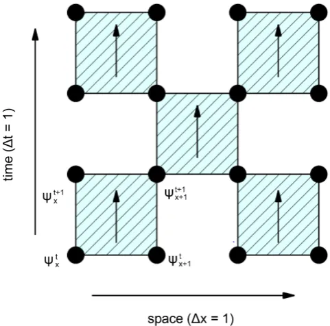
Consider the simplest partitioned QCA on a 1D-time 1D-space lattice of which time evolution rule is given by Figure 1 and Equation (1) (for TDSE-type QCA). This rule is governed by the 2 × _{2 basic unitary matrix (which is called scattering} unitary matrix [11]) which operates on a vector consisting of functions at adja-cent grid points.

( )

1

1 1

1 1 1

cos sin sin cos

t t t

i X i

x x x

t t t

x x x

i

e e

i

θ θ

θ

θ

ψ

ψ

ψ

θ

θ

ψ

ψ

ψ

+

− −

+

+ + +

 ₌   ₌  

      

 

      (1)

Here ≡ _{1 0}0 1

 

X is the x-component of Pauli matrices and 1 1 0 0 1

 

≡    . θ is the parameter of the TDSE-type QCA.

Though it is not straightforward to recognize intuitively, QCA gives a solution of the free particle TDSE in the zero wave number limit

(

k→0

)

.

[image:3.595.253.494.462.700.2]

2

2

1 2 i

t m x

ψ

ψ

∂ _{= −} ∂

∂ ∂ (2) The relation between mass m and θ (the parameter of TDSE-type QCA) is given by

( )

2

(

)

1 t _{tan x: grid spacing, : time step of QCAt}

m x θ

∆ _{= ∆ ∆}

∆ 　　 (3)

This relation can be obtained by several methods as we will mention later. We introduce a simple derivation using FDM for small θ as follows.

By replacing the spatial derivative with the spatial difference, Equation (2) becomes

( )

2 2

1 2 i

t m x

ψ _{δ ψ}

∂ _{≈ −}

∂ ∆ (4)

Here _δ2 _{is the 2nd order central difference operator defined by}

(

)

2

1 1

2 2 2 1

2 1 1

1 2 1

1 2 1

2

1 2 1

1 2 1

1 1 2

S S S S

δ − −

−

 

 

−

 

 ₋ 

  _{ }

≡_ − _ = − + =_{ }

−

  _{ }

 − 

 

 ₋ 

 

(5)

where S is the one-grid shift operator

1 1

1 1

1 1

S

 

 

 

 

≡  

 

 

 

 

 

(6)

(Here we use 6 × _{6 matrices assuming that the system consists of 6-grid points} with periodic boundary condition. Moreover unfilled matrix elements are as-sumed to be zero throughout this article.)

Therefore the time evolution for the time step ∆tFDM is given by

(

)

( )

( )

( )

2 FDM

FDM 2

1

exp where

2 t

t t i t

m x

ψ

+ ∆ ≈

θδ ψ

_

θ

≡ ∆ _

∆

  (7)

This _exp

( )

_iθδ2 _{is approximated according to individual time-discretization}

schemes of FDM. For example the simplest but less accurate scheme is Forward Euler method, where it is approximated as _exp

( )

_iθδ2 _{≈ +1 iθδ}2_{. In QCA}

how-ever _exp

( )

_iθδ2 _{is approximated in a different way. Firstly δ}2 _{is divided into} two parts.

( )

( )

2 2 2

even odd

δ = δ + δ ₍₈₎

( )

2 even 1 1 1 1 1 1 , 1 1 1 1 1 1 δ −    ₋     −  ≡   −    ₋     ₋   

( )

2 odd 1 1 1 1 1 1 1 1 1 1 1 1 δ −    ₋     −  ≡   −    ₋     ₋   

Then _exp

( )

_iθδ2 _{is approximated as a split-step form}

( )

(

( )

)

(

( )

)

(

)

2 2 2

odd even

2

exp exp exp

where cos , sin

i

i i i

c is c is

c is is c

is c c is

e

c is is c

is c c is

is c is c

c s

θ

θδ θ δ θ δ

θ θ − ≈             =                   ≡ ≡ (9)

Note that as

( )

2

( )

2 even

,

odd

δ

δ

have a 2 × _{2 block diagonal form, their} expo-nential can be explicitly calculated. In this way the time evolution for ∆tFDM is divided into two steps ,so we naturally define FDM

QCA ₂

t

t ∆

∆ ≡ _{as the time step of}

QCA and θ is expressed as

( )

QCA2

1 t m x

θ

= ∆

∆ using this definition, which corres- ponds to Equation (3) for small θ.

The QCA dynamics obeys such a simple rule above. However it requires more elaborate techniques to derive the exact relation between mass and QCA para-meter θ in general case Equation (3). This FDM-QCA correspondence is es-sentially the same as the first part of TEBD algorism we discuss later.

π 2

θ

→ limit. Another recent study can be found in [26]. In this study we do

not get into detailed derivation leading to the Dirac equation, as we are interest-ed here in nonrelativistic case, though we will discuss a relevant topic in the last supplementary section.

2.2. Boundary Condition for QCA

There are basically three easily implementable boundary conditions for QCA. These are illustrated in Figure 2. In the cases of (2) (3), the evolution rule at a boundary point(x = 0 or x = N − 1) in odd time is only to multiply the phase ro-tation factor as shown below. (We show only the case x = 0 as the case x = N − 1 is essentially the same).

For zero derivative boundary condition [(2)], phase rotation factor is 1 as

[image:6.595.241.509.277.666.2]

( 1) 1 ( 1) 0 0 1

0 0 0 0

1 1

i X i X

e θ ψ e θ ψ ψ ψ

ψ ψ ψ ψ

−  − ₌ −  _{= ×} _{= ×} − 

       

        (10)

For zero amplitude boundary condition [(3)], phase rotation factor is _e−2iθ _as

( 1) 1 ( 1) 0 2 0 2 1

0 0 0 0

i X i X i i

e θ ψ e θ ψ e θ ψ e θ ψ

ψ ψ ψ ψ

−  − ₌ − − ₌ − − ₌ −  − 

       

        (11)

Note that the unitarity is always satisfied, because the probability increase and decrease are balanced between left and right boundary grid points in the case of (1) and they are zero in the case of (2) (3).

Boundary conditions and discontinuities (inhomogeneities) for QCA are firstly investigated by Meyer. He investigated more general 2-component QCA having two angle parameters. The scalar QCA we use is the simplest one having only one angle parameter, which corresponds to one of factors if his QCA is flattened (namely changed from 2-component to scalar by doubling the number of grid points) and is factorized [23] (2-step QCA of Section 6).

2.3. Multidimensional QCA

It is straightforward to construct multi-dimensional QCA. We have only to use direct product of 2 × _{2 local unitary 1D matrices to generate 2D matrices.}

(

)

2 _{2 ,1 particle case}

U⊗ _{= ⊗}U U D ₍₁₂₎ The rule is illustrated in Figure 3. Concretely

1 1

, , 1 2 , , 1

1 1

1, 1, 1 1, 1, 1

t t t t

x y x y i x y x y

t t t t

x y x y x y x y

c is c is

e

is c is c

θ

ψ ψ ψ ψ

ψ ψ ψ ψ

+ +

+ − +

+ +

+ + + + + +

       

= ⊗

       

  _{    } 

    (13)

(where x, y are even if t is even, and x, y are odd if t is odd.)

As we know each U approximately corresponds to the evolution exp i t _x22

 _∆ ∂ 

 _∂ 

[image:7.595.247.494.495.677.2]

 

or exp i t _y22

 _∆ ∂ 

 _∂ 

 

(

∆t: correspondng time step

)

and they commute with each other, U⊗U approximately corresponds to the evolution

2 2

2 2

exp i t

x y

_∆  ∂ ₊ ∂ 

  

 _{∂ ∂ }

 , namely it causes 2D free TDSE time evolution. We thus generate multidimensional QCA for general dimension.

Applications of QCA to multidimensional cases are studied in [7][8][9]. In multidimensional QW, less straightforward (namely not direct product) models are mainly studied, where the number of internal states is not 2D _{(D: the} di-mension of the space) but less than this (for example 2, 4) [24][25].

2.4. Multiparticle QCA

It is also straightforward to construct (non-interacting) multiparticle QCA. D- dimensional distinguishable M-particle system is equivalent to DM-dimensional 1-particle system. For indistinguishable particle systems, we have to restrict this space to symmetric or anti-symmetric subspace according to the statistics of the particles. Note that _U⊗M _{preserve this symmetry for the case of distinguishable} particle systems and we can define Usvmm⊗M orUasvmm⊗M for the subspace of indis-tinguishable particle systems. (Here U means global unitary matrix, not 2 × ₂ local unitary matrix)Applications of QCA to multiparticle cases are studied in

[3][7][8][9].

3. Second Quantized Form of QCA

3.1. Concrete Evolution Rule of 2nd Quantized QCA

If the one-particle time evolution rule is given by an infinitesimal time evolution matrix, namely, a generator or a Hamiltonian, it is straightforward to construct a 2nd quantized Hamiltonian Hˆ for its free particles.

ˆ

ij ij ij i j

H

_→

H

_≡

_∑

H a a

+

(14)

(Here Hij is the 1-particle Hamiltonian matrix elements, a ai+, j are the creation and annihilation operators for Boson).

If the one-particle time evolution rule is given not by a generator but by a fi-nite time evolution matrix Uij such as in QCA, the construction of its 2nd quantized formalism is done in a slightly different way, which though is consis-tent with the generator case. For example the evolution of 3-particle state

(

U U U

)

ψ

→ ⊗ ⊗

ψ

_{is described as follows}

(

)

(

)(

)(

)

0

0

0 ijk i j k

ijk

ii jj kk i j k i j k ijki j k

i j k ii i jj j kk k ijki j k

a a a

U U U a a a

U a U a U a

ψ

ψ

ψ + + +

+ + + ′ ′ ′ ′ ′ ′

′ ′ ′

+ + + ′ ′ ′ ′ ′ ′ ′ ′ ′

→

=

∑

∑

∑

(15)

Namely we can apply the substitution rule

(

T

)

i i

i _i i i

a

+

U a

+ _′

U a

+ ′ ′

We now apply this substitution rule to 1D free bosonic QCA system where unitary transformation only between nearest neighbor grids occurs, and the one step evolution is given by

( ) ( ) ( ) ( )

(

) (

)

( )

(

) (

)

( )

(

)

0 1 2 3

0 1 _{0 1}

2 3 _{2 3}

0 1 2 3

0 1 2 3

0 1 2 3

0 1 1 0

0 1 2 3

2 3 3 2

1 ₀

! ! ! ! 1 ! ! ! !

0

where cos , sin

n n n n

n n _{i n n}

n n _{i n n}

n n n n

a a a a

n n n n

ca isa ca isa e n n n n

ca isa ca isa e

c s θ θ θ θ + + + + − + + + + + − + + + + + = → + + × + + = =      (17)

The explicit local unitary evolution matrix for the grid pair x=

( )

0,1 _is

(

)

0 1

2 2 2 2 2

2 2 2 2 2

2 2 2 2 2

00 01 10 02 11 20

1 01 10 02 00 2 2 2 2 11 20 i i i i

i i i

i i i

i i i

n n

ce ise ise ce

c e i cse s e

i cse c s e i cse

s e i cse c e

θ θ θ θ

θ θ θ

θ θ θ

θ θ θ

− − − − − − − − − − − − −                             − − −    18)

(local unitary matrices for other grid pairs x=

( ) ( )

2,3 , 4,5  have the same form).

We then apply the substitution rule to 1D free fermionic QCA system. Focus-ing on the grid pair x=

( )

0,1 _{, four states evolve as follows.}

(

)

(

)

(

)(

)

0 0 1

1 1 0

2 2

1 0 1 0 0 1 1 0

0 0

0 0

0 0

0 0 0

i

i

i i

c cc isc e

c cc isc e

c c cc isc cc isc e e c c

θ θ θ θ + + + − + + + − + + + + + + − − + + → → + → + → + + = (19)

Here c0+ and c1+ are fermion creation operators fulfilling anti-commutation

{

c ci+, +j

}

=0. Namely, the local unitary evolution matrix is

0 1

2

00 01 10 11 00 1 01 10 11 i i i i i n n

U ce ise

ise ce e θ θ θ θ θ − − − − −     = _{ }       (20)

It should be noted that if periodic boundary condition is adopted for the grid pair x=

(

N−1,0

)

_{, the off-diagonal element ise}−iθ _{in Equation (20) must be}

replaced with _ise−iθ

( )

₋1M+1 _{considering that}

( )

1 0 1 20 1 0 1 21

M

N N N

c+ n n n n n n

other literatures on multiparticle QCA [3][8][9].

3.2. MPS Approximation of QCA

Now we introduce an interaction between particles. For this purpose, it is reasonable to introduce an additional phase rotation factor by the potential caused by other particles just like the external potential case.

Note that QCA with external potential was firstly studied by Meyer [4]. QCA with the nearest neighbor pair interaction was studied also by Meyer [3]

and Boghosian [8] and Schumacher and Werner [9] in the form we present here.

Here we discuss the simplest case, namely the cases where the nearest neighbor interaction is included. We assume that interaction occurs as an ad-ditional phase rotation only when two particles exist in the neighboring grids. In the context of QLGA (two-component QCA), this additional phase rota-tion corresponds to the phase shift by the collision between the left-going and the right going particles [3]. Under this assumption, the 4 × 4 local unitary evolution matrix becomes

( ) 0 1

2 1

00 01 10 11 1 00 01 10 11 i i i i i n n ce ise U ise ce e θ θ θ θ θ δ − − − − − −     = _{ }         (21)

Here δ>0 meansattraction, and δ<0 means repulsion.

[image:10.595.289.449.335.411.2]

Note that in this simplest case, the structure of evolution scheme is kept same as the structure of free fermion case. After preparing this form, we can apply a MPS approximation and a usual TEBD algorism illustrated by Figure 4 and

Figure 5. A general wave function for the 2nd quantized form of QCA is ap-proximated by MPS as

(

)

( ) ( ) ( ) ( ) ( ) ( ) ( ) ( )

0 1 2 3 4 5 6 7 2nd

0 1 2 3 4 5 6 7 1

0 1 2 3 4 5 6 7

0

, , , , , , ,

m _{n n n n n n n n}

ab bc de

a cd ef fg g

abcdefg

n n n n n n n n

A A A A A A A A

ψ

− =

≈

_∑

(22)

(for the 8 grid points case, m is the dimension of auxiliary spaces and the shape of tensor Ai is (2,m) for i = 0, (m,2,m) for i = 1 to 6, (m,2) for i = 7), then upon the time evolution, each adjacent pair of A A A

(

L, R

)

are updated by applying the 4 × _{4 unitary matrix U of Equation (21) as}

( ) ( )

( ) ( )

1 1 2 1

0 0 0

1 1

0 0

L R L R L R

L R L R

L R

L R

m _{n n} m

n n n n

L ab R bc n n ad d dc

n n b d

m m _{n n}

n n new new

ad d dc L _ad R _dc

d d

A A U V S V

V S V A A

′ ′ ′ ′ ′ ′ ′ ′ − − = = = − − = = = ≈ =

∑ ∑

∑

∑

∑

(23)

[image:11.595.213.535.68.256.2]

Figure 4. MPS approximation of wave function of 2nd quantized QCA and its time evo-lution. This is an example of 8-grid system. A general wave function of the 2nd quantized QCA is represented by a rank-8 tensor. Firstly this rank-8 tensor is approximated by the MPS form (namely by the contraction of 8 low rank (rank-3 or rank-2) tensors). Then the 2nd quantized QCA rule is applied upon the time evolution, namely the contraction with the tensors, four Us (even time) or three Us plus two U1 s (odd time). In this diagram the contraction is assumed to be performed for any connected pair of legs. n n n0, 1 7 represent particle numbers on the grid points.

Figure 5. Time evolution in the TEBD algorithm. When the ten-sor U is applied to the MPS wave function, the original MPS form is destroyed (Left). In order to recover the original MPS form, firstly SVD is applied (Right), then truncate the small sin-gular values which constitutes the part of the contraction “d” so that the dimension of “d” is equal to the dimension of “d”.

For zero derivative or zero amplitude boundary condition, at an odd time, the end points are updated by applying the 2 × _{2 diagonal unitary matrix} U₁.

( ) ( )

(

2

)

1

diag _{U =} 1,1 or 1,_e−iθ _{for zero derivative or zero amplitude}

boundarycon-dition respectively.)

Finally in this section, we compare our method with the ordinal way of reaching the TEBD algorithm. Basically so called hopping term representing ki-netic energy part in evenly-spaced-grid-base (or site-base) quantum models such as Hubbard model or fermionized XXZ model is derived from the FDM-ap- proximation of kinetic energy term. The FDM-approximated Hamiltonian ma-trix of one-particle TDSE is given by

( )

2

(

1

)

1 ₂

2

xx _xx x xx

H S S V

m x δ

−

′ = − − + _′+ ′

[image:11.595.254.495.381.459.2]

(Here Vx is the external potential at the position x.)

And, its 2nd quantized Hamiltonian for non-interacting fermions is

( )

2

(

1

)

( )

2

(

)

ˆ

1 2

xx x x xx

x x x x x x x

xx

xx x

H H c c

M

S S c c V n n c c

m x m x

+ ′ ′ ′ − + + ′ ′ ′ = = − + + + ≡ ∆ ∆

∑

∑

∑

(25)

(The 1st term is so called hopping term. M =

∑

xnx is the total particle num-ber and here we assume it constant).

By adding neighboring interaction term and dropping external potential term and constant term for simplicity, we have fermionized XXZ model [27] [28], where only nearest neighbor grid point of occupation number nx =nx+1=1 have a interaction through δ _.

(

1 1 1

)

_{( )}

2

1

ˆ _{2 where}

2

x x x x x x

i

H c c c c n n

m x

τ

+ +

δ

τ

+ + +     = − + + _ = _ ∆  

∑

(26)

If the anisotropy parameter δ =1_{, this model corresponds to the XXX model} for fermion where the interaction is two-body coulomb interaction.

The XXZ spin model and its equivalent fermionized version are well studied

[27]. The phase diagram of the XXZ spin model in extended systems with the external magnetic field consists of 3 phases, ferromagnetic, paramagnetic and antiferromagnetic phases. When the magnetic field is zero,

1, 1 and 1

δ

>

δ

<

δ

< − correspond to ferromagnetic (gapped), paramagnetic

(gapless) and antiferromagnetic phases respectively and in the paramagnetic phase, quasi particles (magnon) behave as boson-like Tomonga-Luttinger liquid

[29][30]. The magnetic field in the XXZ spin model becomes the chemical po-tential when the model is fermionized. The method has been used for grand ca-nonical systems. We however focus our application in finite system where the number of particles fixed.

According to the TEBD algorism, we decompose the Hamiltonian into two parts.

(

)

(

)

even odd

even 1 1 1 1

:even

odd 1 1 1 1

:odd

2

2

x x x x x x x x

x

x x x x x x x x

x

H H H

H c c c c n n n n

H c c c c n n n n

τ δ τ δ + + + + + + + + + + + + = + = − + − − + = − + − − +

∑

∑

(27)

Time evolution during the small time ∆t _{interval is done as follows} (Suzu-ki-Trotter)

(

)

(

odd

)

(

even

)

exp − ∆i tH ≈exp − ∆i tH exp − ∆i tH (28)

As terms

{

c cx x+ +1+c cx++1 x−nx−nx+1+2δn nx x+1

}

in Heven or Hodd commute with each other, we have

(

even

)

:even

(

( )

(

1 1 1

)

)

exp i tH x exp iτ t c cx x c cx x 2δn nx x + +

+ + +

− ∆ =

∏

∆ + + and

(

odd

)

:odd

(

( )

(

1 1 1

)

)

exp i tH x exp iτ t c cx x c cx x 2δn nx x .

+ +

+ + +

(This is QCA-like evolution). As each factor is finite matrix, we can obtain easily its matrix representation using the standard matrix representation of crea-tion and annihilacrea-tion operator as follows.

( )

01 0 1 1 0 0 1 0 1

0 1

2

00 01 10 11 00 0

01 1 1

10 1 1

11 2 2

H _{c c c c n n n n}

n n

δ τ

δ + +

≡ + − − +

−

 

 

= _ − _

 − 

 

− +

 

(29)

( )

(

)

(

(

)

)

(

( )

)

( )

01 0 1 1 0 0 1 0 1

0 1

2 1

exp exp 2

00 01 10 11 1

00

cos 01

sin 10

11

i i

i i

i

i t H i c c c c n n n n t

n n

c ce ise

s ise ce

e

θ θ θ θ

θ δ

θ δ θ τ

θ θ

+ +

− − − −

− −

− ∆ = + − − + ≡ ∆

 

≡

 

 

= _{  }

≡

 

 

 

 

 

(30)

We see the exact correspondence of the hopping term parameter in the model Hamiltonian τ _{to the QCA parameter} θ, and the strength of correlation in-troduced by δ can be interpreted as the phase factor caused by the local poten-tial at the grid point from the other electron in QCA. When δ =1_{, namely}

( )

2i 1 ₁

e θ δ − _{= , it corresponds to the free Boson approximation case we will address} in the next section.

4. Boson Approximation by Fermionic QCA

4.1. Formalism

As shown in Equation (18) and Equation (20), the grid pair evolution matrix for bosonic QCA is infinite size matrix, whereas that of fermionic QCA is reduced to 4 × _{4. It is desirable if bosonic QCA is well approximated by a QCA with small} degree of freedom as in the fermionic QCA.

We propose here boson approximation by fermionic QCA (or QCA with a hard core condition) when occupation number per grid is small. We mean by the hard core condition that at most one-particle can reside in one grid point. (We not necessarily meanψ

(

x x1, ,2 

)

=0 for

(

xi=xj

)

). We assume that only the amplitudes

ψ

(

x x1, ,2 

)

at points where all

{ }

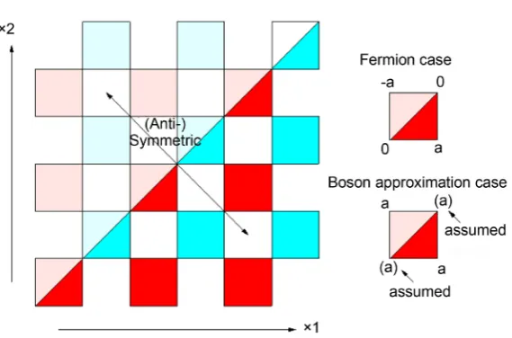
xi are different comprise the full set of independent variables and amplitudes of other points (x1=x2 etc.) needed for evolution are evaluated by interpolation from other points (set to the value of nearby point.) We illustrate in Figure 6 the method of the boson approximation we propose for two-particle case, comparing with free fermionic QCA case.

[image:14.595.231.516.62.250.2]

Figure 6. Fermion or “Boson approximation” in two-particle QCA. We assume that ψ

(

x x1, 2

)

= −ψ

(

x x2, 1

)

for the fermion case, and ψ

(

x x1, 2

)

=ψ

(

x x2, 1

)

for the boson approximation case. Note that even in the boson approximation case, ψ

(

x1=x2

)

is not an independent amplitude and it is interpolated from

other points.

symmetric with respect to exchange of x1 d an x2. And we can obtain the evolu-tion rule at a quadrilateral on the diagonal line as follows.

2 2

2

0 0

0 0

0 0

i i

i

c is c is a c is a c is

e e

is c is c a is c a is c

a e

a

θ θ

θ

− −

−

         

⊗ =

    ₋   ₋  

         

 

 

= _{ }

−

 

(31)

(where we set a=

ψ

(

x+1,x

)

)

For 2-particle Boson approximation case,

ψ

(

x x1, 2

)

must be symmetric with respect to exchange of x1 d an x2, but the amplitude

ψ

( )

x x, cannot be given without some assumptions. We take an approximation to assume that

( )

x x,

(

x 1,x

)

(

x x, 1

)

(

x 1,x 1

)

ψ

=

ψ

+ =

ψ

+ =

ψ

+ + (32)

Under this assumption, we have the following evolution rule.

2i 2i

c is c is _e a a _e c is a a c is a a

is c is c a a is c a a is c a a

θ θ

− −

  _⊗   ₌     ₌ 

           

           

  (33)

This implies, the 4 by 4 Unitary matrix in 2nd quantization formalism changed from that of Fermion case as follows

0 1 0 1

2

00 01 10 11 00 01 10 11

00 1 00 1

01 01

10 10

11 11 1

i i i i

i i i i

i

n n n n

ce ise ce ise

ise ce ise ce

e

θ θ θ θ

θ θ θ θ

θ

− − − −

− − − −

−

   

 _→  

   

   

   

   

(34)

As mentioned before, this 4 × _{4 unitary matrix is the same as that of the} fer-mion system (ferfer-mionized XXZ) with nearest neighbor attractive interaction

1

correspon-dence for this 1D quantum system is easily derived from the QCA-TEBD for-mulation.

We give another possible interpretation of Equation (34). The boson approx-imation Equation (34) can be obtained by applying coarse graining to Equation (18) using the following seemingly reasonable weight matrix for the adjacent grid pair subspace. Namely the 11 - 11 component of Equation (34) (=1) is ob-tained also by

( ) ( )

( )

(

)

2 2

2 2 2 2 2

2 2 2 2 2 2

2 2 2 2 2

1 2 1

1

1, where 2 2 2 , 4

1 2 1

2

2 2

2

ij ij ij

ij

i i i

i i i

ij

i i i

U w U w

c e i cse s e

U i cse c s e i cse

s e i cse c e

θ θ θ

θ θ θ

θ θ θ

− − − − − − − − −     ≡ = _{=  }      −    =_ − _   −  

∑

(35)

Here, coarse graining means that three states of the adjacent grid pair, namely

(

n n0 1

) ( ) ( ) ( )

= 0, 2 , 1,1 , 2,0 , are joined into one state (1,1) so that the occupation number per grid is kept less than 2 upon time evolution. Note that the original bosonic QCA Equation (18) does not conserve hard core condition due to the transition from

(

n n0 1

) ( )

= 1,1 to (0,2) or (2,0).

4.2. Sample Simulation

Here we show examples of the QCA-TEBD application with the boson approxi-mation. In our simulations, we adopt the minimal auxiliary space dimension for MPS which can describe any 1-slater wavefunction (namely 2M _{for M particle} system). 2nd-quantized MPS-form wave function describing 1st-quantized 1- slater wave function 1st

(

)

0, ,1 M 1

x x x

ψ

 ₋ for M particle N grid point system can be given as follows using representation matrices of creation and annihilation operators

(

{ }

ci+ ,

{ }

ci

)

and orthonormal orbitals

(

{

ψi

( )

x

}

)

(i = 0 to M−1: occupied orbital number).

( )

1

_{( )}

0 n _M i i i I A x

cψ x

− =     = _ _ 

∑

 (36)

(

)

(

0

( )

1

( )

1

(

)

)

2nd

0, , ,1 N1 trace 0 1 M 1 n 0 n 1 nN 1

n n n c c c A A A N

ψ + + + −

− = − −

   (37)

We can verify that

(

)

(

)

(

)

( ) ( )

(

)

( )

( )

( )

( )

(

(

)

)

( )

( )

(

)

0 1 1

0 1 1 0 1 1

0 1 1

1st

0 1 1

2nd

1

0 1 1 0 1 1

, 0

0 0 0 1 0 1

1 1

1 0 1 1 1

0

1 0 1 1 1 1

, ,

0 0, 1,0 0, 1,0 0, 1,0 0

trace

M

M M

M

M

x x x

M

M i i i i i i M

i i i

M

M N

x x

M M M M

x x x

n n n

c c c c c c x x x

x x x

x

x x

n M

x x x

ψ ψ

ψ ψ ψ

ψ ψ ψ

ψ

ψ ψ

ψ ψ ψ

For example, in 2-particle case, using the standard representation of Fermion creation and annihilation operators

0

0 1 0 0

1 0 0 1 0 0 0 0

,

0 1 0 0 0 0 0 1

0 0 0 0 c

 

 

   _{  }

=_{  }⊗ _{ }= _

   _{  }

 

1

0 0 1 0

0 1 1 0 0 0 0 1

0 0 0 1 0 0 0 0

0 0 0 0 c

 

 ₋ 

   _{  }

=_{  }⊗ _{ }= _

−

   _{  }

 

we have

( )

( )

( )

( )

( )

0 1

1

0

1 0 0 0 0 1 0 0 0 0 1 0 0 0 0 1

0 0

0 0 0

0 0 0

0 0 0 0

n

A x

x x

x x

ψ ψ

ψ ψ

   

   

   

   

   

   

= _{ }

_{ }

_{ − }

_{ }

_{ }

 

_{ }

 

(39)

We simulated 2-particles in a one-dimensional box using imaginary time evolution.

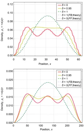
At t = 0 we set 2-particles at adjacent two grid points near the center position. In Figure 7 we show converged density distributions for N = 64,256 and

0,0.95,1

δ = _{cases. For} δ=0 _{(free fermion), it converges to the state where} the two particles occupy the ground and the 1st-exited (1-particle) states.

( )

2 _sin2 πx _sin22πx

n x

N N N

 

= _ + _

  (40)

For δ =1 _{(free boson approximation), it converges to the state where the} two-particle reside in the same (1-particle) ground state.

( )

4_sin2πx

n x

N N

= ₍₄₁₎

Similarly we computed MPS wave function for the three particle system and the results are shown in Figure 8.

In general the parameter of the interaction must be scaled properly when the grid spacing is changed in order to obtain the same continuum limit waveform. It is reasonable that when δ=0 the ground state waveform does not depend on N, and when δ =0.95 _{it depends on} N_{. The case of} δ =1 _{is exceptional in} that the waveform does not depend on N as if the particles were not interacting despite the fact that interaction is taken into account by non-zero parameter. This reflects the validity of the boson approximation.

[image:17.595.233.515.70.504.2]

Figure 7. Converged density distribution of two-particle system (θ=iπ / 4, zero ampli-tude boundary condition). Upper: N = 64 (t = 1500), Lower: N = 256 (t = 20000).

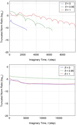
are sufficiently small and MPS approximation must be good for the case. Theo-retically the ratio should be zero for the free fermion case

θ iπ / 4

=

_{, but small}

numerical error is observed.

In Figure 10, we show the converged density distribution

(

)

2 1, 2

x x

ψ of

two-particle system.For the δ =1.0 case, the discontinuity of the wave funcion can be seen at x1=x2. In general the boson approximation wavefuncion

(

1, ,2 3

)

B x x x

ψ

 and the real fermionic wavefunction

ψ

F

(

x x x1, ,2 3

)

are thought to be related by Equation (42) [31].

(

1, ,2 3

) (

1, ,2 3

) (

1, ,2 3

)

F x x x x x x B x x x

ψ

 ≈ 

ψ

 (42)

where



(

x x x

1

, ,

2 3



)

≡

∏

i j>

sign

(

x x

i

−

j

)

.

[image:18.595.239.510.72.491.2]

Figure 8. Converged density distribution of three-particle system (θ=iπ / 4, zero am-plitude boundary condition). Upper: N = 64 (t = 1500), Lower: N = 256 (t =2 0000).

we adopted, though this is not the main purpose of this study. To perform im-aginary time simulation, we set simply θ

(

=τ

( )

∆t

)

_{in the unitary matrix}

Equa-tion (30) to the imaginary value. We performed a canonicalizaEqua-tion of MPS state proposed by Vidal [21] at each simulation step, and in addition to this we per-formed an appropriate gauge transformation of MPS state corresponding to an additional evolution by the spatially constant chemical potential. In a MPS si-mulation of systems of fixed particle numbers, the chemical potential is theoret-ically irrelevant to the result, but it affects the robustness of the simulation and a small numerical error causes violation of particle number conservation leading to the grand canonical ground state.

5. Simulation by 1st Quantized Form of QCA

[image:19.595.242.512.72.509.2]

Figure 9. The ratio of sum of the truncated norms of singular values to that of all singular values in the two-particle system. Upper: N = 64 (t = 0 to 10,000), Lower: N = 256 (t = 0 to 20,000).

[image:20.595.162.539.75.692.2]

(

)

(

)

(

)

(

)

(

)

(

)

(

)

(

)

(

)

1

0 1 0 1

1

0 1 0 1

01 1

0 1 0 1

1

0 1 0 1

2 2 2 2 2 2 2 2 , ,

, 1 , 1

1, 1,

1, 1 1, 1

where t t t t t t t t i

x x x x

x x x x

D U U

x x x x

x x x x

c ics ics s

c is c is ics c s ics

U U e

is c is c ics s c ics

s i θ ψ ψ ψ ψ ψ ψ ψ ψ + + + + −         + +  _{= ⊗}    ₊   ₊       _{+ +}   _{+ +}      −      − ⊗ =_{  }⊗ _{ }= −       −

(

)

(

)

2 2 2

01 2 0 1

1 0 0 0 1 0 0 0

0 0 0 0 1 0 0

if , otherwise

0 0 0 0 0 1 0

0 0 0 1 0 0 0 1

i

i

i

e

cs ics c

e

D x x

e θ θδ θδ −                           = =             (43)

At an even or odd time the evolution rule Equation (43) is applied to each even or odd quadrilateral (namely red or blue quadrilateral in Figure 6) respec-tively. Precisely the rule Equation (43) is for the bulk. At the zero boundaries the application of U in U⊗U are (partially) replaced by the simple phase rotation of Equation (11) at an odd time.

The algorithm of the 1st quantized form of QCA is basically independent of particle statistics. The only procedural difference between boson and fermion is in symmetrization or anti-symmetrization at each simulation step. Without this anti-symmetrization however a decay from a fermionic state to a bosonic state occurs occasionally.

In more general 1D M-particle case, D U U01

(

⊗

)

in Equation (43) becomes

(

∏

i j< D U Uij

)

(

⊗ ⊗ ⊗ U

)

. For example, at the point

(

x x x x0, , ,1 2 3

) (

= 6,7,3, 2

)

in 1D 4-particle case, the additional phase rotation at an even time is _e(2iθδ ×)2 _{which comes from}

(

)

01 0 6, 1 7

D x = x = and

(

)

23 2 3, 3 2

D x = x = _.

In higher dimensional case, the free evolution part

(

U U⊗ ⊗ ⊗ U

)

is the same as in 1D case, and only the paring condition for the additional phase rota-tion need to be modified except for the obvious (anti)-symmetrizarota-tion proce-dure.

In a case of higher dimension or many particles, the requirement for the mag-nitude of θ or δ _{becomes severe. If we set upper bound of phase rotation per} one simulation step to π₂, then 2 π

2 D

θ

≤ is required for the zero boundary

condition and 2

θ δ

(

−1

)

Pmax ≤ π₂ is required. (Here D is the dimension of the space and Pmax is the maximum number of nearest neighbor pairs, especially

max M₂

P = _{for 1D fermion case.)For the more practical programing, we reserve}

the memory only for the simplex region x0 ≥x1≥≥xM−1 taking advantage of the (anti-) symmetry of the wave function though it requires a little bit care.

2D 2 particle fermionic and bosonic systems.

The Hamiltonians related to the fermionic and bosonic QCAs we simulate are

(

)

(

)

2

(

)

F r r r r F r r r r r

rr

H τ c+ c+ c c δ n n n c c+

′ ′ ′

′

 

= −

∑

_ − − + _ = (44)

(

)

(

)

2

(

)

B r r r r B r r r r r

rr

H τ a+ a+ a a δ n n n a a+

′ ′ ′

′

 

= −

_∑

_ − − + _ = (45)

where rr′ _{means nearest neighbor pairs (Note that in 1D fermion case} Equa-tion (44) is the rewritten Hamiltonian of the fermionized XXZ model using

rr′ _).

We show the result of 1D 4 particle and 2D 2particle imaginary time simula-tions in Figure 11 and Figure 12 respectively. We already showed in QCA-TEBD simulation that the fermionic 1D system with δ =F 1 behaves approximately the same as the 1D free bosonic system

(

δ

B=0

)

. More generally, by adding ex-tra phase rotation caused by neighboring grid pair interaction, we conclude that

Figure 11. Converged density distribution of the 1D 4 particle fermionic and bosonic imaginary time simulations.

(

zero amplitude boundary condition

)

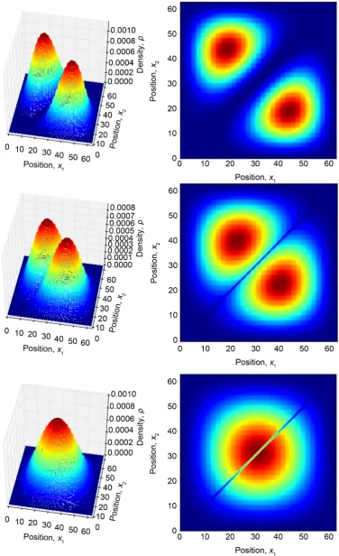
(Upper left: the 2-particle reduced density of the 1D 4-particle bosonic system, Upper right: that of the corresponding bosonic systems, Lower: the 1-particle reduced density. N = 64, δF=0.1 (weak attraction), δB=δF− = −1 0.9 (strong repulsion), t = 1000,

[image:22.595.212.535.298.638.2]

Figure 12. Converged 1-particle reduced density distribution in the 2D 2-particle 1st quantized QCA simulations.

(

zero amplitudeboundary condition

)

(Top and Middle: fermion, Bottom: boson) (N = 64 × 62, δF=2.4 (Top), δF =2.5 (Middle), δB=0

(Bottom), t = 80,000 (Top), 10,000 (Middle, Bottom), θ=iπ 8). At t = 0 we set 2-par- ticles at (x,y) = (32,31) and (31,30). In the process of the time evolution, the bond axis ro-tates from the original 45 to 90 _{. In the fermion case, around 2.5}

F

δ = , there seems to be a transition point to the condensation.

[image:23.595.214.542.77.554.2]

the bosonic system with infinite repulsive delta function behaves as a free fer-mion [31][32]).

By seeing Figure 12 one might expect that fermionic 2D system with δ ≈F 2.5 behaves approximately the same as the 2D free bosonic system

(

δ

B=0

)

, but in more than 1D system, there is no such a simple correspondence between fer-mion and boson as 1D system, because collision points are qualitatively different from boundary points in more than 1D system.

In Figure 13 we show the applicable parameter range of boson approximation in 2/3/4 particle systems. For 1-body-reduced density distribution for bosonic system are well approximated by that of fermionic system when δ ≤F 1. But af-ter δF exceeds 1 the error becomes rapidly larger. For 2-body-(reduced) den-sity distribution, the error increases rapidly when δF reaches slightly below 1. In the condensation state

(

δ

F >1

)

, the assumption used for the wave function interpolation seems to become inapplicable.

6. Multi-Step QCA and Dirac Cellular Automaton

In this supplementary section, we briefly discuss the possibility of multi-step QCA. Firstly we discuss QW and Dirac Cellular Automaton (DCA) [25] [33] [34] as special cases of multi-step QCA. The 1D simplest (namely having only one 2 × 2 unitary matrix as parameters) QW/DCA are mathematically equivalent

Figure 13. Illustration of the applicable range of boson approximation in the 1D 2/3/4-particle case (N = 64, θ=iπ 8, t = 1000). Vertical axis indicates the magnitude of the difference between density distribution of the converged ground states for bosonic and fermionic systems. solid: 1 1

1

B F B

ρ ρ ρ

−

, dotted: 2 2 2

B F B

ρ ρ ρ

−

[image:24.595.213.532.387.639.2]

to the corresponding QCA. This equivalence is easily shown by using the facto-rization form of the two-grid translationally invariant banded unitary matrix (namely multi-step QCA form) [9][23]. In order to interpret QW/DCA as QCA, they are flattened to scalar models as shown in Figure 14.

Namely their two components (up and down) are assigned to two amplitudes of adjacent grid points in the lattice of which the number of grid points are doubled from the original lattice. The 2 × _{2-unit Z-transformation} representa-tion [23] of QCA, QW and DCA are given as

( )

2 1 1 2 1 1 2

QCA 0 ₀

A B A B s A B Cs Ds

U s S S

C D C D s C D As Bs

− − −

−  

         

=    =_  _ = 

        

    (46)

( )

2₂ 2₂ 2 0₂

0

QW

A B A s B s s

U s

C D C s− D s− s−

′ ′

 ′ ′    

=_{  }= _{ }

′ ′

′ ′ _{ }

    (47)

( )

2

DCA 2 1 1

0 0

0 0

s A B s

A s B

U s

s C D s

C D s− − −

′ ′

 ′ ′     

=_{  }= _{  }

′ ′

′ ′ _{   }

  (48)

respectively. Here A B , A B

C D C D

′ ′

   

   _{′ ′}

    are general 2 × 2 Unitary matrices, 2

s is the parameter of the 2 × _{2-unit Z-transformation which means two-grid} shift in the flattened lattice and

( )

2

0 1 0 S s s   ≡  

  is the 2 × 2-unit Z-transfor- mation representation of the one-grid shift matrix defined by Equation (6). Note that _S2_{=s I}2 _{, therefore S}2 _{commute with any 2 × 2 matrix.}

Now we rewrite UQW

( )

s or UDCA

( )

s in a factorization form.

( )

n 0 1 2 n

[image:25.595.63.536.461.676.2]

U s ₌s U SU SU S SU− _{ (49)}

Figure 14. QCA interpretation of QW or DCA. QW or DCA can be interpreted as two-step (U X′ _and X ) QCA. Moreover QW or DCA consists of two independent systems (the cyan system and the magenta system), each of which can be interpreted as sin-gle-step QCA. The correspondence relation between sinsin-gle-step QCA’s U and QW/DCA’s U′ _is U U X= ′ . The only differ-ence between QW and DCA is the definition of the two-component (up and down) state which are indicated by ellipses.

U'

X

U'

U'

X

U'

X

U'

X

U'

X

X

X

X

X

U'

U'

U

t=0

QCA

QW

DCA

time

space space space

Considering 1 1

0 0 1

0 1 0

s _{s XS X}

s − −    _{= ≡}       

     we have

( )

2

(

(

1

)

)

QW

U s ₌s XSXSU− _{′ =} X S XS U− _{′ (50)}

( )

2

(

(

1

)(

1

)

)

DCA

U s ₌s XSU XS− _{′ =}X S U S S XS− _′ − ₍₅₁₎

where U A B

C D

′ ′

 

′ =  _{′ ′}

 . (The expressions in the parentheses of Equations (50) (51) are added in order to clarify the correspondence between the expressions and the graphs in Figure 14.

By taking the logarithm of U s

( )

(see for example [23]) we can obtain TDSE or 1DDirac equation from TDSE-type QCA as its continuum limit. However in this case, obtained 1DDirac equation is not ideal one. In the QW case, the situa-tion is the same. In the DCA case, the more ideal 1DDirac equasitua-tion emerges. In the following we explain the outline of this situation. In the QCA case, we para-metrize the basic 2 × _{2 unitary matrix as follows.}

(

2 2 ₁

)

i A B e C D α β α β

β∗ α∗

  ₌  _{+ =}

  ₋ 

   

 ₍₅₂₎

The corresponding Hamiltonian is

( )

( )

( )

(

)

1 1 log log π 2 i ik s s

H s i U s i e

s s

H s s e

β α α β ∗ − ∗ − −   = = _  _       _′ = −_ + _+ =     (53)

( )

real

( )

_{( )}

1

(

2

)

sink real

k k k

k

s s

H s I

s s

β α

ω ω

ω α β

∗ −

− 

′ ≡ − ∆ = _ _ ∆ =

  (54)

where

( )

(

)

1 real

( )

_{( )}

1

arccos imag ,

sin real k k k s s s s s β α ω β

ω α β

∗ −

− 

−

≡ ∆ ≡ _ _

  (55)

The case Real

( )

β

=0 _(where ω_{k has the form} ( )0 ( )2 2

( )

4

k

k

o k

ω

=

ω

+

ω

+

₎

is particularly simple and important and we restrict our argument to this case.

cos sin cos sin or

sin cos sin cos

i i i

i i i

α β θ θ θ θ

β∗ α∗ θ θ θ θ

     

=

₋     ₋ 

      are the typical cases of

( )

real

β

=0_.

In order to be able to connect this QCA with the Dirac equation, in the wave number

( )

k expansion

( )

2

( )

3

0 1 2

ik

H e′ =H +H k H k+ +o k ₍₅₆₎

0, 1

H H must be traceless (namely their squares are scalar multiples of I) and

0 1 1 0 0

H H +H H = _{which are indeed satisfied. Moreover it would be ideal if}

2 0

H = _{. Although actually} H₂≠0 _{in all cases by similar calculations, only in} the DCA case H2≈0 when k-dependence of _sink

k

ω

DCA more suitable in connecting to Dirac equation.

As we explained above (Equations (50) (51) and Figure 14), the TDSE/Di- rac-type QW/DCA can be regarded as special case of two-step QCA and moreo-ver mathematically equivalent to two sets of TDSE-type single-step QCAs. Therefore the same arguments about the boundary condition, the 2nd quantiza- tion formalism, the simplest interaction and the boson-fermion corresponding as in QCA apparently hold. Moreover in TDSE/Dirac type multi-step QCA the similar argument would be possible, though we need more investigation about what essentially new phenomenon could appear by extending the single-step QCA to the general multi-step QCA (Equation (49)).

7. Conclusion

In this study we show that in one-dimensional multiparticle QCA, the approxi-mation of the bosonic system by fermion (boson-fermion correspondence) can be derived in rather a simple and intriguing way, where the principle to impose zero-derivative boundary conditions of one-particle QCA is also analogously used in particle-exchange boundary conditions. As a clear cut demonstration of this boson approximation, we calculate the ground state of 2 or 3-particle sys-tems in a box using imaginary time QCA-TEBD simulation. Obtained ground states are indeed boson-like. We also perform imaginary time simulations by the 1st quantized form of QCA not only for fermionic system but also for bosonic system and show the applicable range of boson approximation (boson-fermion correspondence

(

δ

B =

δ

F −1

)

). Another point we want to emphasize through-out this study is that QCA, TEBD (MPS), FDM are deeply related to each other. The 1st quantized form of QCA can be regarded as the split step decomposition of FDM description for TDSE, which is essentially the same approximation used when TEBD algorithm is obtained from the model quantum Hamiltonian sys-tem with nearest neighbor interaction. On the other hand, the 2nd quantized form of QCA has the TEBD form from the beginning.

Acknowledgements

This work was supported by Education Center for Next-generation Simulation Engineering, Toyohashi University of Technology and University-Community Partnership Promotion Center, Toyohashi University of Technology. We would like to thank Prof. Hitoshi Goto for his support and Dr. Akira Saitoh for his helpful advice.

References

[1] Wiesner, K. (2009) Quantum Cellular Automata. In: Meyers, R.A., Ed., Encyclope-dia of Complexity and Systems Science, Springer, New York, 7154-7164.

https://doi.org/10.1007/978-0-387-30440-3_426

[2] Grössing, G. and Zeilinger, A. (1988) Quantum Cellular Automata. Complex Sys-tems, 2, 197-208.