Angular Impulse and Spinning Bouncing Ball

http://www.scirp.org/journal/wjm ISSN Online: 2160-0503

ISSN Print: 2160-049X

Angular Impulse and Spinning Bouncing Ball

Haiduke Sarafian

1

_{, Nanaz Lobe}

2

1_{The Pennsylvania State University, University College, York, PA, USA} 2_{Merck & Co., Inc., Kenilworth, NJ, USA}

Abstract

A solid ball of mass m, size r and spin ω about an axis through its center is dropped freely from a height h on a rough horizontal plane. Assuming its an-gular momentum is parallel to the horizontal plane upon impact it bounces repeatedly drifting on a vertical plane. We analyze the kinematics of the bouncing ball assuming the impacts are semi-elastic without slipping. By va-rying the spin and relevant parameters, a robust Mathematica [1] program enables simulating the trajectories.

Keywords

Bouncing Spinning Ball, Linear Impulse, Angular Impulse, Computer Algebra System, Mathematica

1. Introduction

Kinematics, including multiple trajectories of a bouncing massive point-like par-ticle on a vertical plane thrown at an angle with respect to a horizontal surface is a classic physics problem [2]. The point-like character of the object i.e. the lack of its size suppresses the impact of its internal degrees of freedom, e.g. spin, on kinematics. We depart from this stepping stone scenario and consider a genera-lization where a point-like object is replaced with a round shaped entity such as a solid and/or a hallow ball or a short length cylinder. The spin adds interesting features to the kinematics. For instance a free falling spinning object upon im-pact with a horizontal surface bounces multiple times drifting away from the points of impacts. As we were developing the mathematics of the problem aux-iliary quantities such as: run-time between adjacent bounces, sensitivity of the range between sequential bounces and etc. were calculated as well. The general features of these analyses are summarized in a Mathematica based simulation program making the analysis robust providing opportunities exploring the “what if” scenarios. This note is composed of three sections. In addition to Mo-How to cite this paper: Sarafian, H. and

Lobe, N. (2017) Angular Impulse and Spinning Bouncing Ball. World Journal of Mechanics, 7, 177-183.

https://doi.org/10.4236/wjm.2017.77016 Received: June 21, 2017

Accepted: July 9, 2017 Published: July 13, 2017

Copyright © 2017 by authors and Scientific Research Publishing Inc. This work is licensed under the Creative Commons Attribution International License (CC BY 4.0).

http://creativecommons.org/licenses/by/4.0/

tivation and goals, in Sect. 2 we develop the needed physics solving the problem. This section also embodies analysis and output. Section 3 is the conclusions and closing remarks.

2. Physics of the Problem and Its Solution

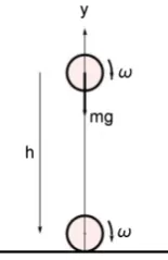
Figure 1 depicts the scenario at hand. A solid ball of mass m, size r and clock-wise spin ω about the horizontal axis through the center is held, h, distance away from a horizontal reflecting surface. The ball is dropped freely, as it falls the only active force on the ball is the weight that passes through the center; this pre-serves the spin from the point of release to the impact, as shown.

At the impact the floor imparts three different effects: 1) it reorients the initial downward vertical velocity in a slanted upward direction 2) because of surface roughness it generates a horizontal impulse drifting the ball along the horizontal, specifically, it pushes the ball along the opposite direction of the orientation of the angular velocity at the impact, x-axis as shown in Figure 2(b) and 3) the surface roughness slows the spin. These are depicted in Figure 2.

It is intuitive to say that right after the bounce because gravity is the only ac-tive force acting on the ball the center of the ball would trace a parabolic trajec-tory. Furthermore, because of the same reason the spin of the ball stays the same; its angular momentum conserves. One may also extend the aforementioned conclusions for all subsequent multiple bounces the number of which is deter-mined by the restitution factor, e.

With this intuitive insight to quantify the kinematics we formulate the prob-lem.

[image:2.595.334.412.464.584.2]

We write the dynamic version of the Newton’s law as,

[image:2.595.281.467.622.704.2]

Figure 1. A spinning ball held at rest from a re-flecting surface.

( )

(

)

2 1 2 1 d t t

t t=m −

∫

N v v , (1)

where N

( )

t is the floor reaction and is perpendicular to the interface.

Sym-bolically speaking the time span,

(

t2−t1

)

, is the contact time of the ball-floor

and its value depends on the value of e. For the analysis of the problem on hand its value doesn’t come in the play. The v1 and v2 are the corresponding

ve-locities right before and after the impact, respectively. By projecting Equation (1) along the x-axis and replacing the integrand with

µ

sN

( )

t i.e. the maximum static friction we identify the cause of the horizontal push. In this scenario the RHS of Equation (1) is, v1x =0 and momentum of the drifted bounced ball is mv2x. Accordingly, Equation (1) along the x-axis is,

( )

2 1 2 d t s x t

N t t mv

µ

_∫

= , (2)

one may realize the integral on the Left Hand Side (LHS) is the linear impulse along the y-axis. Note also the orientation of the static friction shown in Figure 2(a) is the cause of spin retardation. Its impact is given via angular impulse. Writing Equation (1) for the torque and related angular momentum gives,

( )

(

)

2 1 1 2 d t cm t

t t I

τ

=

ω ω

−

∫

, (3)

where

τ

( )

t is the torque, so that the LHS is the angular impulse, where I_cm is

the moment of inertia of the rotating object about the center-of-mass (cm) and ω’s are the associated spins, i.e. angular velocities. Applying Equation (3) to the case on hand replaces the integrand with r

µ

sN t

( )

, yielding,

( )

(

)

2 1 1 2 d t s cm t

r_µ N t t_=I ω ω−



∫

 , (4)

Substituting Equation (2) in (4), gives,

(

2x

)

cm

(

1 2

)

r mv =I

ω ω

− , (5)

Furthermore, while the ball is in contact with the floor and rolls without slip-ping we apply, v=r

ω

. Specifically, for the problem on hand the horizontal

component of the velocity, v2x, right after the bounce is subject to v2x=rω2.

Substituting this in Equation (5) we get,

2 2 1

1 1 cm mr I ω ω             = +

, (6)

Accordingly, we realize the explicit relationship between the spins before and after the impact; i.e., 0<ω2<ω1, meaning 1) the bounced ball spins slower after

2

cm

I =

γ

mr . Depending to the character of the object on hand, e.g. a solid

sphere, a hallow sphere or a short cylinder about its axial axis, γ, is known. These are γ = 2/5, 2/3 and 1/2, respectively. Substituting for Icm, Equation (6) yields,

2 1 1 γ ω ω γ   =  ₊ 

  . (7)

its value for a solid ball is, ω2=2 7ω1. That is a free falling solid sphere

irrespec-tive of the mass, size and the initial height, h, upon impact loses 71% of its spin. In general the ball bounces more than once. Following analysis similar to the aforementioned reveals the subsequent bounces don’t alter the spin other than the first bounce; i.e. the spin given by Equation (7) stays the same. This is justi-fied according to Equation (5). For a multiple bounce it reads,

(

fx ix

)

cm

(

i f

)

mr v −v =I ω ω− , (8)

where i and f indicate the “initial/before” and “final/after” states. For a rolling ball we substitute vix =rωi and

v

fx

=

r

ω

f , Equation (8) yields,

ω ω

i

=

f .

Meaning the static friction doesn’t do mechanical work and preserves the spin. This is the same conclusion that one draws analyzing the states of a rolling ball on a rough horizontal surface. An auxiliary outcome of this observation is the equality of the horizontal velocities between the multiple bounces. However, be-cause the runtimes between the bounces dependent on the restitution factor, e, their associated range, i.e. the horizontal traveled distances between adjacent bounces differ. Perfect elastic collisions with e=1 result identical range.

For instance, the runtime between the first and the second impact is,

2 2h

t e

g

= _.

During this time interval v2x=rω2. Combining the latter two expressions

with Equation (7) yields,

1

range 2 2

1 h r e g γ ω γ   =  ₊ 

  . (9)

Its value for a solid ball with γ =2 5 is, 1

4 2 7 h r e g

ω . Without proof this is

mentioned in [3].

Having considered the aforementioned information we derive analytic equa-tions describing the trajectories of a spinning bouncing ball. In the coordinate system depicted in Figure 2, after the first bounce because the gravity is the only active force the center of the ball traces a parabolic trajectory [2],

( )

(

2

( )

)

2

( )

2 2

1 tan tan

2

g

y x x x

v θ θ

= − + + _{, (10)}

(

)

2

2 2

2 1 2

1

v r γ ω e gh

γ

   

=_{   } +

+

 

  , (11)

( )

1 2 tan 1 gh e r θ γ _ω γ =    ₊   

In these equations g is the gravity, the takeoff speed after the first impact is v2,

the projectile (reflected) angle is θ, h is the initial height and the restitution fac-tor is, e.

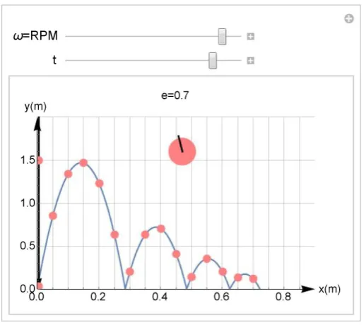
Utilizing this information we craft a Mathematica code simulating the features of a spinning bouncing elastic ball. Accordingly, as shown in Figure 3 for two chosen values; h = 3.0 m, and e = 0.7 with two control sliders we adjust the ini-tial spin, ω, and the number of the bounces with the t-slider. A real-life anima-tion of this program traces the bounces according to the running “ω clock” de-picted with the pink disk-clock and its single arm. This figure shows the charac-ters of a bouncing ball with e = 0.7. Running the program with e = 1 results mul-tiple parabolas with the same heights.

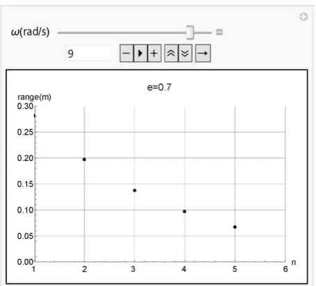
Auxiliary information about the quantities of interest such as range, Equation (9), for a chosen initial spin ω vs. the number of the bounces is shown in Figure 4. With this program one has the capability of simulating the sensitivity of the range as a function of ω.

[image:5.595.245.503.475.705.2]

For instance as shown, a spinning ball with ω = 9 rad/s dropped form a 3.0 m height drifts 27.9 cm between the first and the second impact; 19.6 cm between the second and the third and etc.

Figure 5 shows the variation of the reflecting angle θ vs. spin value ω. Equa-tion (12) is used plotting this graph. One might have intuitively expected this; however, this graph quantifies the output. The initial heighth, e factor and γ used in this plot are, 3 m, 0.7 and 2/5, respectively.

Figure 5 shows the fast spin corresponds to a smaller reflection angle and vi-sa-versa. For instance, a slow spinning ball with ω = 10 rad/s ~ 100 rev/min bounces almost vertically. Yet, a fast spinning ball with ω = 100 rad/s ~ 1000 rev/min reflects at 62˚ with respect to horizontal.

[image:6.595.260.488.68.274.2]

Figure 4. Plot of the range vs. number of the bounces for a chosen e value; here e = 0.7.

Figure 5. Display of the bounced angle θ vs. the spin ω.

3. Conclusion

[image:6.595.235.511.323.489.2]

restitution factor e and 3) the number of the bounces. Additional auxiliary quan-tities such as the reflection angle, range and etc. are also quantified. All the graphs and quantified values reported here in our investigation are produced using Mathematica [1] software and its accompanied text [4] and guidelines ex-plained in a recently published book [5].

References

[1] Mathematica™ (2015) Is Symbolic Computation Software, V11.0, Wolfram Research Inc.

[2] Halliday, D., Resnick, R. and Walker, J. (2014) Fundamental of Physics. 10th Edi-tion, Wiley and Sons, New York.

[3] Lawden, F.D. (1967) A Course in Applied Mathematics. The English Universities Press Ltd., London, EC4, 239.

[4] Wolfram, S. (1996) Mathematica Book. 3rd Edition, Cambridge University Press. [5] Sarafian, H. (2015) Mathematica Graphics Example Book for Beginners. Scientific

Research Publishing. http://www.scirp.org

Submit or recommend next manuscript to SCIRP and we will provide best service for you:

Accepting pre-submission inquiries through Email, Facebook, LinkedIn, Twitter, etc. A wide selection of journals (inclusive of 9 subjects, more than 200 journals)

Providing 24-hour high-quality service User-friendly online submission system Fair and swift peer-review system

Efficient typesetting and proofreading procedure

Display of the result of downloads and visits, as well as the number of cited articles Maximum dissemination of your research work