Towards Understanding the Normalization in Structural VAR Models

Munich Personal RePEc Archive

Towards Understanding the

Normalization in Structural VAR Models

Kociecki, Andrzej

National Bank of Poland

17 June 2013

Online at

https://mpra.ub.uni-muenchen.de/47645/

T

OWARDS

 

U

NDERSTANDING

 

THE

 

N

ORMALIZATION

 

IN

 

S

TRUCTURAL

 

VAR

 

M

ODELS

 

Andrzej Kocięcki

National Bank of Poland 

e–mail: andrzej.kociecki@_nbp.pl

First version: November 2012 

This version: November 2012

Abstract: The aim of the paper is to study the nature of normalization in Structural VAR models. Noting that normalization is the integral part of

identification of a model, we provide a general characterization of the

normalization. In consequence some the easy–to–check conditions for a

Structural VAR to be normalized are worked out. Extensive comparison

between our approach and that of Waggoner and Zha (2003a) is made.

Lastly we illustrate our approach with the help of five variables monetary

Structural VAR model.

I.

I

NTRODUCTION

The great merit of Waggoner and Zha (2003a) and Hamilton et al (2007) is

that they made us realize how subtle the normalization in Structural VAR (SVAR)

models is. That is contrary to the common view normalization can influence the small

sample probabilistic inference in an uncontrollable and strange way. Poor

normalization can lead to multimodal small sample distributions of maximum

likelihood estimates or multimodal posterior distributions (of function) of parameters

of interest. This phenomenon will manifest itself in a rather inaccurate description of

statistical uncertainty.

The reaction to the normalization puzzle in SVAR models was the so–called

likelihood preserving (LP) normalization proposed by Waggoner and Zha (2003a).

sign of each equation, the likelihood possesses a multitude of global modes. In order

to make the probabilistic statements reliable we should choose one mode and focus on

the shape of the likelihood in the appropriate area around this mode (we should not

mix “contents” of two or several modes in terms of their statistical uncertainty).

Our position is different. We take seriously the statement of Hamilton et al.

(2007) that “the normalization problem is fundamentally a question of identification”.

Although Waggoner and Zha (2003a) motivated and justified their normalization rule

in the context of well–behaved impulse response functions (IRF’s), our contribution is

the remark that ill–behaved IRF’s are consequence of the lack of global identification.

Building on this we proposed different normalization rule whose primary role is to

achieve this global identification. The merit of our normalization rule is that it is

mathematically deduced straight from the very basic definition of normalization. On the other hand the LP normalization is based on informal reasoning (though it

possesses some desirable properties). Moreover our normalization is ordinal. That is

we lay down a priori permissible sign for a subset of coefficients in the

contemporaneous matrix. In contrast using the LP normalization we sometimes

multiply coefficients in a given equation by 1 but sometimes by minus 1 (depending

on what is closer to the mode).

We offer theoretical insight (which is contrary to the common understanding)

that sometimes it is not sufficient to restrict the sign of one coefficient in every

equation to normalize a model. As we will show in non–recursive SVAR models we

usually need more sign restrictions. In fact this may be also perceived as the

significant contribution of our paper since at this level of the SVAR model design the

economic theory must enter the scene e.g. you must take a stand a priori on whether supply is downward or upward sloping.

It turns out that our normalization also sheds some new light on more and

more popular sign restrictions used to identify the impact of some shocks in a SVAR,

see e.g. Uhlig (2005). Although it is well understood that using only sign restrictions

is insufficient to identify a model we claim that they may be necessary for

identification. That is according to our theory sign restrictions may constitute

inevitable part of the identification of a model i.e. without them a model may be

unidentified even if the conditions given in Rubio–Ramírez et al. (2010) are met.

Since the articles of Waggoner and Zha (2003a) and Hamilton, Waggoner and

Zha (2007) are frequently cited in the sequel they will be referred to as WZ and

II. G

ENERAL

D

EFINITION OF

N

ORMALIZATION IN

SVAR

M

ODEL The subject of this paper is to understand the nature of normalization in the

following SVAR model

1 1

t t t p p t

y A′ = +c y A′₋ + +y′₋ A +ε′; for t =1,…,T (1)

where A: (m×m) is the nonsingular matrix of contemporaneous relations between the data y_t : (m×1), A_i : (m×m), c : (1×m) is a vector of constants and

1 2 1

| , , (0 , I )

t yt yt N m m

ε _{− −} … ∼ _× . Let us define B′=[c′A1′…Ap′]. Further let Om denote

the space of (m×m) orthogonal matrices i.e. { m m | I }

m m

O = g ∈ × g g′ =gg′= .

Assume that restrictions identify a SVAR model up to arbitrary sign of each

equation. Let us denote this restricted parameter space as , r A B

Θ . To distinguish the identification up to arbitrary sign of each equation from the concept of global

identification we term the former as the regional identification. The label “regional”

prompts that this is more than local property. Formally

Definition 1: The SVAR is regionally identified at ( , ) r_, A B

A B ∈ Θ if and only if (ifif)1

, { | ( , ) , } r

A B m A B

S = g ∈O Ag Bg ∈ Θ =D, where D ={diag( ,...,δ₁ δm) |δi = ±1}.

Following the literature we confine ourselves to the normalization put only on

elements of A. Hence we restrict permissible A’s to some subset n m m A

×

Θ ⊂ which

entails inequalities on some entries in A matrix. It just amounts to augmenting , r A B

Θ with inequality constraints n

A

Θ . Let R be the space of all regionally identified parameter points such that n

A

A∈ Θ i.e. {( , ) , |

r n

A B A

R = A B ∈ Θ A∈ Θ and ( , )A B is regionally identified} . Of course we must assume that R ≠ ∅. Hence we have intuitively clear

Definition 2: A normalization is a subset Θ ⊂n_A m m× such that for all ( , )A B ∈R we

have { | ( , ) , , } {I }

r n

m A B A m

g ∈O Ag Bg ∈ Θ Ag ∈ Θ = .

1

Hence to normalize a model means to achieve global identification on R (uniformly). That is when a normalization is imposed the point that is regionally identified

becomes globally identified.

Let ( , )A B ∈R. Since

, ,

{ | ( , ) r , n} { | ( , ) r } { | n}

m A B A m A B m A

g ∈O Ag Bg ∈ Θ Ag ∈ Θ = g ∈O Ag Bg ∈ Θ ∩ g ∈O Ag ∈ Θ

We obtain by definition 1

,

{ | ( , ) r , n} { | n}

m A B A m A

g ∈O Ag Bg ∈ Θ Ag ∈ Θ =D∩ g ∈O Ag∈ Θ ⊆D (2)

Hence equivalent definition of normalization is

Definition 2A: A normalization is a subset Θ ⊂n_A m m× such that for all ( , )A B ∈R we

have { | ( , ) , , } {I }

r n

A B A m

g ∈D Ag Bg ∈ Θ Ag∈ Θ = .

WZ refer to “conventional” normalization as the sign choice of arbitrary

(nonzero) element in each equation. With the help of simple 2–dimensional recursive

model they demonstrate that “conventional” normalization may entail apparent ill–

behavior of the probability statements for impulse responses. Since this example

constitutes the motivation to develop “appropriate” normalization rule by WZ we

first analyze this example from our perspective (which is complementary to that

adopted by WZ). To this end we ignore any lags in SVAR since they do not play any

role in our reasoning. Consider the simple SVAR y At′ =εt′, where

11 21 22

0 a A=⎡⎢_{a a} ⎤⎥

⎢ ⎥

⎣ ⎦ i.e. 0

r A

⎡ ⎤

Θ = ⎢ ⎥

⎢ ⎥

⎣ ⎦. Evidently I2

r A

∈ Θ and

2

I { 2 | I2 } r A

S = g ∈O g ∈ Θ =D. Hence the model

is regionally identified at A=I2. As noted by WZ if we employ the normalization

that all diagonal elements in A are positive i.e. { 2 2 | 11 0, 22 0} n

A A a a

×

Θ = ∈ > > ,

which leads to { r | n} r n 0

A A A A

R A A

+ +

⎡ ⎤

⎢ ⎥

= ∈ Θ ∈ Θ = Θ ∩ Θ = _{⎢ ⎥}

⎣ ⎦, then I2

r n

A A

∈ Θ ∩ Θ and

2 2 2

{ | I r n} {I }

A A

g ∈O g ∈ Θ ∩ Θ = i.e. the model is globally identified at A=I₂. Using the “conventional” normalization argument we could replace n

A

Θ with

2 2

21 22

{ | 0, 0}

n

A A a a

×

Θ = ∈ > > , which induces { r | n}

A A

R= A∈ Θ A∈ Θ = 0

r n

A A + +

⎡ ⎤

⎢ ⎥

= Θ ∩ Θ =

⎢ ⎥

⎣ ⎦. WZ show how strange results may appear when normalization

n A

Θ is used. However to point out clear unreasonableness of normalization n A

identified using n A

Θ ceased to be so with n A

Θ . Hence using n A

Θ we “lose” from potentially normalized (globally identified) set some regionally identified points. The

general question is this: Is it reasonable to sacrifice some points from globally

identified set when they are economically reasonable? This suggests that the

arbitrariness of “conventional” normalization is illusory and must be abandoned.

Formal analysis is calling for.

Using definition 2 we have a useful alternative characterization of

normalization

Proposition 1: A normalization is a subset n m m A

×

Θ ⊂ such that for all ( , )A B ∈R;

1

{I }

n

A m

D∩A−Θ = , where 1 n { 1 | n}

A A

A−Θ = A A A− ∈ Θ .

Proof: Let ( , )A B ∈R. We have { | ( , ) , , }

r n

m A B A

g ∈O Ag Bg ∈ Θ Ag ∈ Θ =

{ | n}

m A

D g O Ag

= ∩ ∈ ∈ Θ by (2). We shall prove { | n}

m A

g ∈O Ag ∈ Θ =

1

{ | n}

m A

g O g A−

= ∈ ∈ Θ . We get

n A

Ag ∈ Θ ⇒ Ag =A for some n

A

A∈ Θ ⇔g =A A−1 for some n A

A∈ Θ ⇒ 1 n

A

g ∈A−Θ On the other hand

1 n A

g ∈A−Θ ⇒ g =A A−1 for some n A

A∈ Θ ⇔Ag =A for some n

A

A∈ Θ ⇒ n

A

Ag ∈ Θ Then for arbitrary ( , )A B ∈R

1 1

,

{ | ( , ) r , n} { | n} n

m A B A m A m A

g ∈O Ag Bg ∈ Θ Ag ∈ Θ =D∩ g ∈O g ∈A−Θ =D∩O ∩A−Θ =

1 n A

D A−

= ∩ Θ

The result follows by replacing { | ( , ) r_, , n}

m A B A

g ∈O Ag Bg ∈ Θ Ag ∈ Θ with 1 n

A

D∩A−Θ in definition 2.

Proposition 1 is the most general and valid for all kinds of homogenous restrictions (i.e. linear or nonlinear, whether the restricted parameter space is

variation free or not etc.). However if the restricted parameter space is variation free

i.e. when restrictions on A and B are independent of each other, then more intuitive

and easily checkable condition is available (see below). Proposition 1 says that a

model is normalized ifif for all ( , )A B ∈R the only common element of the two subsets D and 1 n

A

A−Θ is the identity matrix. In principle, to achieve this global identification we must have that ( , )∀ A B ∈R, 1 n

A

A−Θ is a subset with all diagonal elements strictly greater than minus one (since D={diag( ,...,δ1 δm) |δi = ±1}).

However even in very special cases this is not feasible e.g. when A is lower triangular

must ensure that ( , )∀ A B ∈R, 1 n A

A−Θ is a subset with strictly positive diagonal elements. Using proposition 1 we automatically rule out cases when A is singular

and/or 1 n

A

A−Θ is empty. The very reason for this is that our definition of normalization is uniform i.e. it has to be fulfilled for all ( , )A B ∈R.

In the rest of paper we focus on the case when ,

r r r

A B A B

Θ = Θ ×Θ i.e. restricted parameter space is variation free so as the restrictions on A and B are independent

of each other. This covers unquestionably the most common use of SVAR model in

which restrictions are confined to A matrix only. The main reason for that is to have

a close contact with WZ (and to be concise).

Anyway though in general case our starting point to study normalization

would be proposition 1, when ,

r r r

A B A B

Θ = Θ ×Θ we have

Proposition 2: Suppose Θr_{A B,} = Θ ×Θr_A r_B. If ∀( , )A B ∈R; ∩ −1 Θ ∩ Θ =

( r n) {I }

A A m

D A

then n A

Θ is a normalization, where −1(Θ ∩ Θ =r n) { −1 | ∈ Θ ∩ Θr n}

A A A A

A A A A .

Proof: First note that given ,

r r r

A B A B

Θ = Θ ×Θ we have

,

{ | ( , ) r , n} { | r n, r}

A B A A A B

g ∈D Ag Bg ∈ Θ Ag∈ Θ = g ∈D Ag ∈ Θ ∩ Θ Bg ∈ Θ =

{ | r n} { | r}

A A B

D g D Ag g D Bg

= ∩ ∈ ∈ Θ ∩ Θ ∩ ∈ ∈ Θ

Analogously as in the proof of proposition 1 we can show { | r n}

A A

g ∈D Ag ∈ Θ ∩ Θ

1

{ | ( r n)}

A A

g D g A−

= ∈ ∈ Θ ∩ Θ . Hence

1 ,

{ | ( , ) r , n} ( r n) { | r }

A B A A A B

g ∈D Ag Bg ∈ Θ Ag∈ Θ =D∩A− Θ ∩ Θ ∩ g ∈D Bg ∈ Θ

Note that if r_, r r

A B A B

Θ = Θ ×Θ then { r n, r |

A A B

R= A∈ Θ ∩ Θ B ∈ Θ ( , )A B is regionally identified}. Let A B, ∈R be arbitrary. It follows

1 ,

{ | ( , ) r , n} ( r n) { | r }

A B A A A B

g ∈D Ag Bg ∈ Θ Ag∈ Θ =D∩A− Θ ∩ Θ ∩ g ∈D Bg ∈ Θ

If 1( r n) {I }

A A m

D∩A− Θ ∩ Θ = then { | ( , ) , , } {I }

r n

A B A m

g ∈D Ag Bg ∈ Θ Ag ∈ Θ = since

∈ ∈ Θ

{ | r}

B

g D Bg is non–empty and contains I_m. This proves that n

A

Θ is a

normalization.

Proposition 2 gives sufficient condition for normalization when ,

r r r

A B A B

Θ = Θ ×Θ and there are some restrictions imposed on B. However if the restrictions are confined to

A only, then proposition 2 constitutes necessary and sufficient condition for

normalization. For future reference let us denote rn r n

A A A

Θ ≡ Θ ∩ Θ .

A normalization consistent with proposition 2 will be refereed to as PL

normalization (you can think of PL as an abbreviation for “plain” or alternatively as

is appropriate when restricted parameter space is variation free and requires that for

all ( , )A B ∈R, the only common element from two subsets D and 1 rn A

A−Θ is the identity matrix. This will be achieved by the condition that all elements in 1 rn

A

A−Θ have strictly positive diagonal elements. In the important special case when all

restrictions are confined to A only we must ensure that for all A∈Θrn_A such that A is regionally identified, 1 rn

A

A−Θ has strictly positive diagonal elements. Or simply for

every , rn

A

A A∈ Θ , 1

A A− has strictly positive diagonal elements.

The inevitable question from which we could not escape is how PL

normalization looks like when using recursive SVAR models i.e. A is lower or upper

triangular and B unrestricted. It is easy to note that restricting all elements on the

diagonal of A to be positive or negative works well. Let us show this. Without loss of generality assume A is lower triangular with positive diagonal elements. Then 1

A− is lower triangular with positive diagonal elements too. If we postmultiply 1

A− by any A, which is also lower triangular with positive diagonal elements, then a product

1

A A− is lower triangular with positive diagonal elements. Lastly the only common element of D and the space of lower triangular matrices with positive elements is the

identity matrix.

III. F

IRST

I

LLUSTRATION OF

PL

N

ORMALIZATION

As a first illustration of our approach we use the example of orange demand

and supply discussed in detail in HWZ. Let yt′ =( , ,q p wt t t), where qt denotes the log

of the number of oranges sold in year t, pt is the log of the price and wt is the

number of days with below–freezing temperatures in year t. The model is as follows

11 12

21 22 1 1

31 33

0 0 0

t t t p p t

a a

y a a c y A y A

a a

ε

− −

⎡ ⎤

⎢ ⎥

⎢ ⎥

′_{⎢ ⎥} = + ′ + + ′ + ′

⎢ ⎥

⎣ ⎦

(3)

where A_i’s are unrestricted. Of course the restricted parameter space is variation free

hence proposition 2 applies. First equation represents a supply, second – a demand

and the last one depicts the exogenous process w_t. One may show that the model (3)

is regionally identified almost everywhere [Lebesgue] (in fact provided that 11 12

21 22

a a a a

⎡ ⎤

⎢ ⎥

⎢ ⎥

⎣ ⎦ is

nonsingular and a31 ≠0). By assumption A must be also non–singular hence

33 0

11 12 21 22 31 33 0 0 0 a a A a a

a a ⎡ ⎤ ⎢ ⎥ ⎢ ⎥ = ⎢ ⎥ ⎢ ⎥ ⎣ ⎦ ⇒ 1

A− =

22 33 12 33 1

21 33 11 33

31 22 31 12 11 22 21 12

0

[det( )] 0

a a a a

A a a a a

a a a a a a a a

− ⎡ ₋ ⎤ ⎢ ⎥ ⎢ ⎥ ⋅ − ⎢_{− −} ⎥ ⎢ ⎥ ⎣ ⎦

where det( )A =a a a_{11 22 33}−a a a_{33 12 21}.

Let 11 12 21 22 31 33 0 0 0 a a A a a

a a ⎡ ⎤ ⎢ ⎥ ⎢ ⎥ = ⎢ ⎥ ⎢ ⎥ ⎣ ⎦

be arbitrary. Then diagonal elements of 1

A A− are given as

11 ( 22 33 11 12 33 21)/( 11 22 33 33 12 21)

d = a a a −a a a a a a −a a a

22 ( 11 33 22 21 33 12)/( 11 22 33 33 12 21)

d = a a a −a a a a a a −a a a (4)

33 ( 11 22 33 21 12 33)/( 11 22 33 33 12 21)

d = a a a −a a a a a a −a a a

Our goal is to guess n A

Θ such that for every , rn A

A A∈ Θ , 1

A A− has strictly positive diagonal elements i.e. d_ii >0; ∀i. It is easily verified that taking n

A

Θ to be the space of A’s with strictly positive diagonal elements is insufficient to complete the global

identification of the model. We need one more assumption: a12 is positive and a21 is

negative (or vice versa). Interestingly this requires economic reasoning. Since the first

equation is a supply and the second is a demand it is natural to assume a21 <0 and

12 0

a > (note that all coefficients of each contemporaneous relation are on the left side in SVAR (1))2_{. Hence}

11 22 33 21 12

{ | 0, 0, 0, 0, 0}

n m m

A A a a a a a

×

Θ = ∈ > > > < > (5)

Imposing PL normalization allows us to postmultiply (3) by 1 1 1 11 22 33

( , , )

diag a− a− a− to get (with some abuse of notation)

1 1

1 0

1 0 0 1

t t t p p t

y c y A y A u

h

η

γ _{− −}

⎡ ⎤ ⎢ ⎥ ⎢ ⎥ ′_{⎢ ⎥} = + ′ + + ′ + ′ ⎢ ⎥ ⎣ ⎦ (6)

Note that with PL normalization η =a12/a22 >0, γ =a21/a11 <0, h =a31/a11 and 2 2 2

3 1 11 22 33

(0 , ( , , ))

t

u ∼N _× diag a− a− a− . The notation used in (6) is not accidental. The specification (6) “almost” corresponds to the so–called η−normalization in HWZ.

2

We wrote “almost” since η−normalization in HWZ does not take into account the sign restrictions η>0 and γ <0, which are in fact necessary for global identification. The interesting fact about (6) under the PL normalization is that it

roughly conforms to the so–called identification principle i.e. normalization rule

proposed by HWZ. Identification principle applied to (6) says that boundaries for

allowable entries of A matrix should correspond to the loci along which the log

likelihood is −∞. In our case this locus is γη =13_{. Although the locus of γη =1 is}

not on the boundary of the parameter space in (6) what PL normalization does

instead is to exclude the parameter points for which γη =1 holds (since η>0 and 0

γ < ).

To illustrate all these issues we simulated the sample of 100 observations from

1

1 0.1 0 0.2 0.5 0 0.1

0.5 1 0 0.12 0.3 1 0.1

0.5 0 1 0.3 0 0.1 0.4

t t t

y y₋ ε

′

⎡ ⎤ ⎡ ⎤ ⎡ ₋ ⎤

⎢ ⎥ ⎢ ⎥ ⎢ ⎥

⎢ ⎥ ⎢ ⎥ ⎢ ⎥

′_⎢− _⎥ =_{⎢ ⎥} + ′ _{⎢ ⎥}+ ′

⎢ ⎥ ⎢ ⎥ ⎢ ⎥

⎣ ⎦ ⎣ ⎦ ⎣ ⎦

; εt ∼N(0 , I )3 1× 3 (7)

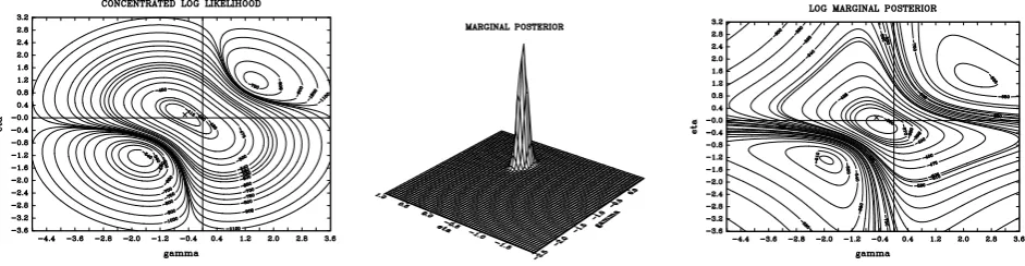
Since a_ii =1 for i =1,2, 3; we have a₁₂ ≡ =η 0.1, a₂₁ ≡ = −γ 0.5 and a₃₁ ≡ =h 0.5. The first picture in Figure 1 shows the contours of concentrated log likelihood for η

and γ evaluated at the true values for h =0.5 and a_ii =1, for i =1,2, 3. The true values of η and γ are marked with “×”. The likelihood has one global maximum and two local peaks (of unequal height). The areas of great concentration of the

contour levels correspond to the loci along γη =1 (at which the log likelihood approaches −∞). Using the PL normalization we restrict the support to the second quadrant i.e. η>0 and γ <0. Thus we automatically exclude parameters along and in the vicinity of γη =1 that are situated both in the first and the third quadrant. It is instructive to find out how these problems carry over into the posterior results.

Although the multimodality naturally characterizes the marginal posterior of η and

γ (derived under the flat prior for all parameters in SVAR), see the last picture in Figure 1, the contribution of these modes to the visible shape of the posterior is none,

see the middle picture in Figure 1. The reason is that the ratio of the height of the

marginal posterior of η and γ at the global maximum to that of the second largest

peak (around γ = −2, 1.2η = − ) is about 150

e . In consequence the IRF’s computed

from (6) even without inequality constraints η>0 and γ <0 are well behaved too

3

i.e. the error bands for IRF’s are not too wide and quite conclusive, see HWZ.

However in contrast to HWZ we interpret these results differently. For HWZ the

parameterization (6) without inequality restrictions η>0 and γ <0 is acceptable since “for practical purposes it is sufficiently close […] to a true identification–based

normalization”. As we will show in section VI, this conclusion is case–sensitive. In

this particular 3–dimensional SVAR subject to the particular identifying scheme,

restricting the diagonal elements in A results in well behaved posterior of parameters

and its functions e.g. IRF’s. In general this is not a rule. In fact this is the message

from WZ. Using the PL normalization guarantees well behaved posteriors of

parameter and its functions in larger models when the simple visual inspection of the

shapes of the likelihood and/or posterior is not readily available and ad–hoc

normalization rules are not an option.

Quite obviously those inequality constraints turn out to be also sign

restrictions for impulse responses. For example instantaneous response of the price to

a one standard deviation positive shock to a quantity supplied is

12 a a12 33/(a a a11 22 33 a a a33 12 21)

ϕ = − − . Using PL normalization we have ϕ₁₂ <0.

Moreover the instantaneous effect of a one standard deviation increase in quantity

demanded on the price is strictly positive under PL normalization (since

22 a a11 33/(a a a11 22 33 a a a33 12 21) 0

ϕ = − > ). This ensures that we avoid all pitfalls

connected with “conventional” normalizing rules which were convincingly illustrated

[image:11.595.59.530.515.637.2]

in Figure 4 in HWZ.

Figure 1: From the left: a) contours of concentrated log likelihood of γ and η evaluated at the true value of h=0.5 and the diagonal elements in A matrix i.e. aii =1 for i=1, 2, 3; b) marginal posterior of γ and η under the flat prior for all

parameters in SVAR; c) contours of the log marginal posterior of γ and η under the flat prior for all parameters in SVAR.

IV. S

UFFICIENT

C

ONDITION FOR

PL

N

ORMALIZATION In our example of the orange demand–supply, n

A

Θ turns out to be equivalent

to assumption that rn

A

A

provided that the restricted parameter space is variation free this requirement is all

we need to complete the global identification of SVAR model.

Among basic model assumptions is that det( )A ≠0. Commonly this assumption was thought as unimportant because the set of singular matrices has zero

Lebesgue measure. For instance using Bayesian simulation methods to estimate

SVAR, in practice we could not encounter a draw which entails singular A. However

the theoretical importance of the singularity of A has been recognized and discussed

by WZ and HWZ. The message from these both articles is that the permitted

parameter space should exclude the subspace on which the likelihood vanishes. The

goal of this section is to demonstrate that the latter informal statement can be

formally justified.

To proceed further we need one more notation. Given two matrices X =( )xij

and ( )Y = yij of the same dimension we write X ≤cY if xij ≤yij for each ,i j. Hence

“≤_c” denotes component–wise inequality. We have

Proposition 3: Assume ,

r r r

A B A B

Θ = Θ ×Θ . Let A and A be given matrices in Θr_A.

Assume that rn { r | }

A A A A c A c A

Θ = ∈ Θ ≤ ≤ is such that each A∈ Θrn_A is nonsingular. Then for every A∈ Θrn_A , A−1Θrn_A is a subset with strictly positive diagonal elements.

Proof: This is the application of theorem 1.2 in Rohn (1989), which states that

under hypothesis of our proposition, 1 1 2

A_∗ =A A− , for every 1, 2 rn A

A A ∈ Θ , is the so– called P −matrix (a square matrix A_∗ is the P −matrix if all its principal minors are positive). In particular since each diagonal element is the principal minor, the

proposition follows.

Needless to say some entries in A may be set to ∞ and that in A to minus ∞. Proposition 3 forms a basis for useful sufficient condition to achieve global

identification. One has to derive analytically det( )A . If it happens that imposing inequalities on some or all entries in A restricts the latter so as det( )A >0 or

det( )A <0 then setting rn { r | det( ) 0}

A A A A

Θ = ∈ Θ > or rn { r | det( ) 0}

A A A A

Θ = ∈ Θ <

will complete the identification of a model. The choice between

{ | det( ) 0}

n

A A A A

Θ = ∈ Θ > and n { | det( ) 0}

A A A A

Θ = ∈ Θ < depends on the model at

hand (but is only illusory, see right below). Thus instead of finding n A

Θ such that

rn A

A

∀ ∈ Θ ; 1 rn A

elements of A in the form A≤_c A≤_c A so as det( )A >0 or det( )A <0. Note that derivation of det( )A even in large SVAR model is usually not very difficult. This is

because of many zero restrictions imposed on A. In fact prior to derivation of

det( )A , we can permute the rows and columns of A so as there appear blocks of

zeros (which usually simplify derivation of det( )A ). The permutation operation is

permissible since it only changes the sign of the determinant but both det( )A >0 and det( )A <0 restriction is acceptable.

Note that when A is lower or upper triangular (or its subset) then if diagonal

elements of A are restricted to be positive we immediately get det( )A >0. This justifies our conviction that the correct normalization is the same for recursive and

non–recursive model provided that we follow the rule to restrict A so as det( )A >0.

V. C

OMPARISON OF

PL

N

ORMALIZATION TO

LP

N

ORMALIZATION

It is instructive and desirable to compare our theory with the LP

normalization proposed by WZ. The first step to apply LP normalization is the

derivation of the maximum likelihood (ML) estimator of A to be denoted as ˆA.

Proposition 4: Assume that r_, r r A B A B

Θ = Θ ×Θ . Suppose there is a mode A in ˆ rn A

Θ . Then the PL normalization implies the LP normalization restricted to rn r

A B

Θ ×Θ . Proof: PL normalization implies that for every two distinct , rn

A

A A∈ Θ , A A−1 must have strictly positive diagonal elements. Since a mode ˆA belongs to rn

A

Θ it follows that for every rn

A

A∈ Θ , 1ˆ

A A− has also strictly positive diagonal elements. The latter is the LP normalization.

Otherwise, if we operate on ,

r r r

A B A B

Θ = Θ ×Θ (and not on rn r

A B

Θ ×Θ ), the LP and PL normalizations are incomparable notions. However if ˆ rn

A

A∈ Θ , by proposition 4, any

rn A

A∈ Θ is consistent with the LP normalization. On the other hand the parameter points that are chosen using the LP normalization may not belong to rn

A

Θ 4_{. Thus as a}

general principle we may expect that error bands for IRF’s in a model under PL

normalization will be narrower than those in a model under the LP normalization.

4

Consider the model of the orange demand–supply from section III. Let us focus on the first diagonal element of 1_ˆ

A A− . Suppose aii=1;∀i, a12=0.1 and a21=0.2 (note that a21 violates the PL normalization). Further suppose that ML estimators are aˆ11=1 and aˆ21= −0.1. Then the first diagonal element of

1_ˆ

A A− is

Utilizing the PL normalization we may hope for more clear–cut economic conclusions

as far as IRF’s are concerned. That this hope is justified will be illustrated in section

VI.

Without loss of generality assume rn { r | det( ) 0}

A A A A

Θ = ∈ Θ > . Then we have

the following

Proposition 5: Assume that ,

r r r

A B A B

Θ = Θ ×Θ . Suppose rn { r | det( ) 0}

A A A A

Θ = ∈ Θ >

entails the inequalities so as proposition 3 holds. Let Γ =diag(γ₁₁,…,γ_mm) be any matrix with γ_ii ∈[0,1]. Then for all , rn

A

A A∈ Θ we have det(AΓ +A(I_m− Γ >)) 0.

Proof: By assumption 1

det(AΓ +A(I_m− Γ =)) det( ) det((IA ⋅ _m − Γ +) A A− Γ). Then det(AΓ +A(I_m − Γ >)) 0 ifif 1

det((I_m − Γ +) A A− Γ >) 0. By theorem 1.2 in Rohn (1989), for all , rn

A

A A∈ Θ , 1

A A− is a P−matrix (hence all principal minors of

1

A A− are positive). Proposition follows by expansion of 1

det((I_m− Γ +) A A− Γ) by the diagonal (I_m− Γ) (see e.g. Seber (2008), pp. 61–62 or Harville (1997), p. 196) and noting that for every Γ and , rn

A

A A∈ Θ , the determinant is positive.

In particular under hypothesis of proposition 5 and provided that ˆ rn A

A∈ Θ we get det(AˆΓ +A(I_m − Γ =)) det([γ11 1aˆ + −(1 γ11) ,a1 …,γmm maˆ + −(1 γmm)am])>0 for all

[0,1]

ii

γ ∈ , where ˆa_i denotes the i−th column of ˆA and a_i that of A. In contrast the LP normalization works column–wise so as given a1…ai−1,ai+1…am, we choose ai

such that det([ ,a1 …,ai−1,γaˆi + −(1 γ) ,a ai i+1,…,am])>0, for all γ ∈[0,1], i.e. ˆai and

i

a lie on the same side of the hyperplane { m | det( ) 0,

i

a ∈ A = given

1 i 1, i 1 m}

a …a− a+ …a . Evidently the PL normalization ensures that ˆai and ai lie on the

same side of the hyperplane but simultaneously for all i=1,…,m and unconditionally (i.e. without conditioning on a1…ai−1,ai+1…am).

VI. A

M

ONETARY

P

OLICY

E

XAMPLE

As a second (real–data) example we consider a monetary SVAR proposed by

Kim (1999). The contemporaneous matrix A is restricted as follows (B unrestricted) MP MD PS PS Inf

A= log log log log c R M P Y P

11 12 15 21 22 25 32 33 35 42 43 44 45

51 55

0 0 0 0

0 0

0

0 0 0

a a a

a a a

a a a

a a a a

The identifying scheme is quite similar to that used in Waggoner and Zha (2003b)

(except that (8) does not include unemployment). The model includes 5 variables: the

federal funds rate (R), logarithm of the monetary aggregate M2 ( logM ), logarithm of

the consumer price index ( logP), logarithm of the real GDP interpolated on a

monthly frequency and logarithm of the Commodity Research Bureau price index for

raw industrial commodities (logP_c). Each column in (8) represents a behavioral

equation that is signified at the top. “MP” stands for monetary policy (or money

supply) equation and “MD” stands for money demand. Equations labeled with “PS”

succinctly describe production sector and “Inf” stands for the information market.

We employed the US dataset used in Waggoner and Zha (2003b), which is

available at http://www.tzha.net/computercode (where detailed description of the data may be also found). The data are monthly and cover 01.1959–12.2000.

By theorem 7 in Rubio–Ramírez et al. (2010) the model under the identifying

scheme (8) is exactly identified i.e. globally identified almost everywhere. In our

language it means that we can define the set of regionally identified parameter points.

Since the restricted parameter space is variation free, to get complete identification

we need to impose the PL normalization. To this end we use proposition 3 and we

have to derive the determinant of A. We easily get

det( )A =a a a_{∗ 44 55} −a₄₄(a a a a_{51 22 33 15}−a a a a_{51 12 33 25})

where a∗ =a a a11 22 33−a a a33 21 12. Kim (1999) implicitly assumed that all diagonal

elements in A are strictly positive. However it is not sufficient for global

identification (i.e. PL normalization). We need to find inequalities on the parameters

so as det( )A >0. Hence in addition to aii >0 (i=1,…, 5), we must assume that

21 12 0

a a < , a a_{51 15} <0 and a a a_{51 12 25} >0. To use proposition 3 we must derive from the last three inequalities the implied inequalities for single elements. This should be in

principle assisted by the economic theory. Using standard economic reasoning since

the second equation is money demand we assume a12 >0 (by assumption a22 >0 and

we use a convention that all contemporaneous variables are on the left in SVAR).

Moreover a21 <0 is also reasonable since we can think of the first equation as money

supply (note that we also assume a11 >0). Since Pc is the commodity price index in

dollars we should expect that monetary authority should increase the interest rates

when world commodity price rises. Hence a51 <0. Then we must assume a15 >0 to

fulfill a a51 15 <0. With these choices we must also restrict a25 <0 (so as

51 12 25 0

equation as “an arbitrage equation which describes a kind of financial market

equilibrium”. Thus in case of large economy (like US) domestic interest rates and

money aggregates may affect P_c through the direct pressure on world commodity

price. When the interest rate rises in large economy it should have tendency towards

lowering the commodity prices. That is a15 >0. Moreover when the money aggregate

increases in large economy there is a natural pressure to increase the commodity

prices, hence a25 <0. Needless to say the above inequality restrictions put on A give

rise to sign restrictions for IRF’s (at least for immediate responses).

We estimated the model with p =12 lags using Bayesian approach. To this end we used the flat prior for A and B in order to preserve the likelihood shape.

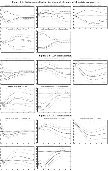
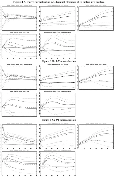
Figures 2 and 3 present IRF’s of all variables to a one standard deviation

contractionary monetary policy shock and a money demand shock, respectively. These are shocks identified with the first two equations. The solid line presents the

IRF evaluated at the maximum likelihood (ML) estimators of A and B. The dashed

line (usually very close to the solid one) is median response, two “dots–dashes” lines

cover 68% of the posterior probability (point–wise). Lastly two dotted lines are 90%

posterior probability bands. In each figure a panel A shows results using naïve

normalization i.e. diagonal elements in (8) are positive, panel B demonstrates the

output using LP normalization and panel C – the PL normalization.

The ML estimates imply IRF’s expected by economists. For instance, the

interest rate rises and a money falls initially, the real GDP declines quite quickly

reaching the minimum within half a year and consumer prices decline persistently.

Since error bands are meant to describe uncertainty around “mean” response, the

probabilistic conclusion may not be so certain and depends on how you normalize the model. With naïve normalization the matter is hopeless which was already nicely

demonstrated in WZ. We found out nothing about the most important aspects of the

monetary policy shock i.e. its impact on interest rate, real GDP and consumer prices.

In general probability bands of all IRF’s are suspiciously wide. As we emphasized this

is a consequence of the methodological fault and not the “uninformativeness” of the

data. Adoption of the LP normalization results in more conclusive probability

statements for IRF’s. However the question of great importance is how LP and PL

normalizations differ from each other and whether these differences are economically

important. Firstly using the PL normalization we get particularly well determined

IRF of the interest rate to a monetary policy shock. We are quite certain that the

anticipation of falling prices and by realizing by monetary policy decision makers that

output has already declined). In contrast the analogous IRF using the LP

normalization gives an ambiguous impression5_{. Secondly with the PL normalization}

we definitely get rid of the “price puzzle” i.e. prices move up after a contractionary

monetary policy shock. In this respect probabilistic conclusions are much sharper

with PL normalization than LP normalization.

In fact in all cases PL normalization makes the probabilistic statement more

informative than when employing the LP normalization. Sometimes it is not a critical

difference but sometimes it is economically crucial (e.g. compare the response of

consumer prices to a money demand shock).

VII. C

ONCLUSION

Our goal was to properly grasp the notion of normalization in SVAR models. Using basic definition of normalization in SVAR models we proposed the easy

working condition for normalization in SVAR models when the restricted parameter

space is variation free. It was called the PL normalization. We emphasized that

normalization is an integral part of the identification of SVAR. To put it another

way, only properly normalized parameter point becomes globally identified.

We compared our theory to the likelihood preserving (LP) normalization

proposed by Waggoner and Zha (2003a). Our basic attitudes to normalization are

quite different. We maintain that a correct approach is to trace the overall shape of

the likelihood of the globally identified model whereas Waggoner and Zha (2003a)

focus on its shape in the close area around the mode in a model which is “almost”

identified (up to arbitrary sign of each equation). In our opinion a proper

normalization is not a matter of appropriate description of uncertainty around the maximum likelihood estimate of IRF (as suggested by Waggoner and Zha (2003a)),

but is the last and necessary step towards achieving the global identification of

SVAR model.

However our theoretical findings are in line with the recommendation of

Waggoner and Zha (2003a) and Hamilton et al. (2007) to put the parameter points

which imply the zero likelihood or failure of local identification on the boundary of

5

the parameter space. On the other hand we disagree with Waggoner and Zha (2003a)

claim that “the correct normalization for recursive models turns out to be, in general,

inappropriate for nonrecursive models”. Our conclusion is that the correct

normalization is the same for recursive and non–recursive SVAR provided that we

fully understand what the normalization is (the appropriate normalization rule is the

same).

We demonstrated theoretically and in practice that using PL normalization we

get narrower IRF’s error bands than when employing the LP normalization. Hence

the PL normalization may be welcomed by applied macroeconomists as it will tend to

confirm more firmly their intuition.

Although general nonlinear identifying restrictions may make the

normalization irrelevant (see e.g. Waggoner and Zha (2003a)) there is an important

class of nonlinear restrictions (e.g. short–run and long–run impulse response restrictions) that also require normalization rule. Though we provided useful

characterization of normalization in such a case (see proposition 1) we really did not

study it and leave these aspects of normalization for future research.

REFERENCES:

Hamilton, J.D., D.F. Waggoner and T. Zha (2007), “Normalization in Econometrics”, Econometric Reviews, 26, pp. 221–252.

Harville, D.A. (1997), Matrix Algebra from a Statistician’s Perspective, Springer–Verlag, New York.

Kim, S. (1999), “Do Monetary Policy Shocks Matter in the G–7 Countries? Using Common Identifying Assumptions about Monetary Policy Across Countries”, Journal of International Economics, 48, pp. 387–412. Rohn, J. (1989), “Systems of Linear Interval Equations”, Linear Algebra and Its Applications, 126, pp. 39–78. Rubio–Ramírez, J.F, D.F. Waggoner and T. Zha (2010), “Structural Vector Autoregressions: Theory of

Identification and Algorithms for Inference”, The Review of Economic Studies, 77, pp. 665–696. Seber, G.A.F (2008), A Matrix Handbook for Statisticians, John Wiley & Sons, Inc., Hoboken, New Jersey. Uhlig, H. (2005), “What Are the Effects of Monetary Policy on Output? Results From an Agnostic Identification

Procedure,” Journal of Monetary Economics, 52, pp. 381–419.

Waggoner, D.F., and T. Zha (2003a), “Likelihood Preserving Normalization in Multiple Equation Models”, Journal of Econometrics, 114, pp. 329–347.

[image:19.595.74.511.71.761.2]

Figure 2 A: Naive normalization i.e. diagonal elements of A matrix are positive

Figure 2 B: LP normalization

[image:20.595.71.510.72.758.2]

Figure 3 A: Naive normalization i.e. diagonal elements of A matrix are positive

Figure 3 B: LP normalization