A simulation method to estimate task specific uncertainty in 3D microscopy

1

A simulation method to estimate task-specific

uncertainty in 3D Microscopy

3

Giovanni Moroni

_{, Wahyudin P. Syam}

_{, and Stefano Petrò}

1 _{School of Mechanical Engineering, Tongji University, Cao An Road, 201804 Shanghai, P.R. of China} 5

2 _{Mechanical Engineering Department, Politecnico di Milano, Via La Masa 1, 20156 Milan, Italy} 6

3 _{Manufacturing Metrology Team, Faculty of Engineering, University of Nottingham, NG7 2RD,} 7

Nottingham, UK

8 9

Corresponding author: Wahyudin P. Syam ([email protected]) 10

11

Abstract:

12

Traceability in micro-metrology requires an infrastructure of accredited metrology 13

institutes, effective performance verification procedures, and task specific uncertainty 14

estimation. Focusing on the latter, this paper proposes an approach for the task specific 15

uncertainty estimation based on simulation for a generic 3D microscope. The proposed 16

simulation approach is based on the identification and a successive parameter 17

estimation of an empirical model of measured points. The model simulates the probing 18

error of the 3D microscope based on a Gaussian process model, thus including the 19

correlation among close points. Parameters for the error simulation are estimated by a 20

deep analysis of error sources of the 3D microscope. Validations of the proposed 21

simulation approach are carried out in the case of focus variation microscopy (FVM), 22

considering several case studies. The procedure proposed in the ISO/TS 15530-4 23

standard are applied for validation. 24

25

Keywords: Uncertainty, 3D microscopy, geometrical metrology, micro-metrology, 26

ISO/TS 15530-4, focus-variation. 27

28

1. Introduction

29

Micro-engineered components are important since they can integrate functions and 30

intelligence into products [1]. These products need micro-geometrical metrology to 31

verify their compliance to tolerances. Coordinate measuring systems (CMSs), being 32

suitable for micro-geometrical metrology are in most cases non-contact (optical) 33

instruments, due to their flexibility in accessing the surface of parts, elimination of the 34

risk of damaging small and delicate micro features and fast data acquisition rate [2]. 35

Among the others, 3D microscopy (3DM) seems very promising and already counts a 36

lot of industrial applications, particularly in the field of surface analysis. 3DM gathers 37

technique like coherence scanning interferometry, phase shifting interferometry, 38

confocal scanning microscopy, confocal chromatic microscopy, digital holography, and 39

focus variation microscopy. Most 3DM techniques are based on the sequential 40

acquisition of images of the sample, while changing the distance between the sample 41

and the objective lens. 42

43

1.1 Measurement traceability and uncertainty 44

Regardless of the considered measuring instruments, traceability of measurements is 45

very important for a reliable measurement result in the case of micro-geometrical 46

metrology as well. Traceability requires not only periodical instrument performance 47

2 or according to some predefined performance indexes, but also measurement 49

uncertainty must be stated to guarantee measurement comparability [3]. The subject of 50

performance verification has been addressed by the authors in previous papers [4, 5]: 51

this paper addresses the problem of the uncertainty estimation. 52

The main reference for measurement uncertainty estimation is the “Guide to the 53

expression of uncertainty in measurement” (GUM) [6]. According to the GUM, when 54

a final measurement result comes from several distinct measurement data processes, 55

the uncertainty is derived based on the propagation of the uncertainty from each 56

uncertainty contributor along the data processing chain, thus GUM requires a closed 57

form mathematical model of the measurement. In addition, for coordinate metrology, 58

measurement uncertainty is “task-specific” [7], i.e. a single measuring instrument can 59

perform several different measurement tasks with different measuring strategies, which 60

are characterized by a different uncertainty [8]; hence the GUM method is difficult to 61

apply. 62

The ISO 15530-3 [9] and ISO/TS 15530-4 [10] standards propose alternative methods 63

to effectively estimate the measurement uncertainty for coordinate metrology. The ISO 64

15530-3 method needs expensive calibrated artifacts; hence it is not suitable when a 65

product has many variants, as it would require many different calibrated artifacts, or 66

when small production volume cannot justify the cost of a calibrated artifact. The 67

ISO/TS 15530-4 simulation method seems more promising in the case of high product 68

or high demand variability. The main drawback of the simulation method is its 69

computational intensity [11], but the continuous reduction of computational costs 70

should reduce this issue. 71

72

1.2 Simulation approaches 73

A simulation-based approach seems to be the most promising solution to estimate a 74

task-specific measurement uncertainty, especially for optical-distance sensor 75

instruments, as suggested by Evans [11] in the case of interferometry. Baldwin et al. 76

[9] used a simulation approach to estimate the uncertainty in tactile-CMM 77

measurement. They simulated CMM geometric errors and incorporated them in the 78

kinematic model of the CMM, so that the nominal position of points could is modified. 79

Kruth et al. [12] proposed a similar approach, with addition of part form deviation as 80

an uncertainty source. Cheung et al. [13] also used a similar approach to estimate the 81

uncertainty in the case of free-form surface measurements. All these simulation 82

approaches neglect the presence of spatial correlations among the sampled points. 83

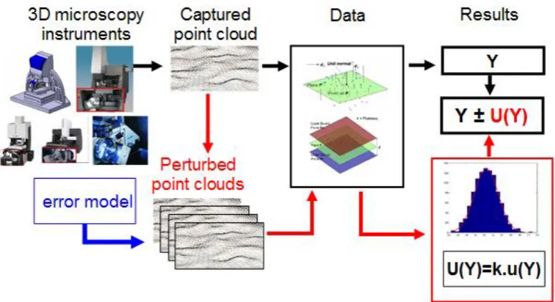
In general, a simulation approach relies on a point perturbation process (an error 84

simulator) generating a perturbation of a reference cloud of points, as shown in Figure 85

1. Detailed explanation of the framework applied to CMMs was described by Trapet 86

and Waldele [14]. The scheme consists of two paths, the first one (Figure 1: black 87

arrow) estimates a measurement result Y, while the second one (Figure 1: red arrow) 88

estimates the measurement uncertainty U. The first path is explained as follows: a point 89

cloud is obtained by the selected measuring system using a defined measuring strategy. 90

This point cloud is then processed to calculate the measurement result Y. The second 91

path starts from the same sampled point cloud. A point perturbation process by 92

measurement error simulation is applied to the original point cloud. The perturbed point 93

cloud is processed by the same numerical algorithm that is gathered to the measurement 94

result and the results are stored. The simulation of the error is repeated for an adequate 95

number of times (usually a few thousand) and the simulated measurement results are 96

stored. The estimated uncertainty usim (U = 2 usim) of a measurement is the sample 97

3 99

Figure 1: Framework a simulation method for the uncertainty estimate. 100

101

1.3 Research aim 102

In this paper, a simulation-based approach considering spatial correlation among 103

points is proposed. The proposed model does not directly take into consideration 104

physical phenomena related to interactions between materials and light; rather the 105

model includes the effect of the physical interaction between the materials and the light 106

inside several uncertainty sources, e.g. material types, and parameters of the simulation. 107

There are several technical reasons behind this consideration. First, even if well-108

established physical models exist for the interaction between electromagnetic waves 109

and matter, their application is numerically impractical to apply and to the degree of 110

accuracy required for 3DM measurement simulation. In general, the intensity value on 111

each single pixel is not completely independent of the others. Hence, a single ray 112

coming to the complementary metal-oxide semiconductor (CMOS) sensor has some 113

degree of correlation with its neighbor ray of light [15]. And finally, some techniques 114

add an additional contribution to the correlation among points, as the optimization 115

function allowing the identification of the coordinates of the single point is calculated 116

considering the neighboring pixels, selected by a windowing process [15]. 117

Hence, to empirically model this phenomenon, the basis of the methodology is a 118

Gaussian process [16], in which data are randomly distributed according to a 119

multivariate Gaussian distribution, whose covariance structure depends on the spatial 120

distribution of points. The multivariate Gaussian process can capture and simulate the 121

correlation among points. 122

This paper is structured as follows. Section 2 describes the mathematical model 123

allowing the simulation of the correlated points. Section 3 introduces Focus Variation 124

Microscopy (FVM) as technology considered for the validation of the approach, and 125

then focuses on the estimation of the parameters required to run the simulation. Finally, 126

section 4 validates both the model and the estimation of the parameters according to the 127

ISO/TS 15530-4 standard. 128

2. Task-specific uncertainty estimation by simulation in 3DM

129

The proposed approach relies on a point perturbation process (an error simulator) 130

4 as shown in Figure 1. A correlation means that the error behavior of a point depends on 132

other points within a certain distance from it. The simulation approach (figure 1, blue 133

box) uses a Gaussian process model completely defined by a variogram function, we 134

call it “variogram error model”. The need of this kind of model arises from how a 3DM 135

measurement is taken. As explained in section 1.3, it is expected that the measurement 136

errors of the single sampling points are not independent but correlated. An independent 137

simulation of them could then lead to a simulation far from the reality. The use of a 138

Gaussian process described by a variogram error model allows the simulation of non-139

independent measurement errors, coherently with the measurement method. 140

141 142

2.1 Mathematical model for the simulation of a perturbed cloud of points 143

The core of the uncertainty estimation by simulation is the model for the perturbation 144

of the point cloud. In general, the perturbation of the cloud of points is given 145

x, y, z

  

   , which are rotation errors with respect to x, y and z axes, and x, y, zi.e.

146

linear errors along x, y and z directions, respectively. Once these perturbations have 147

been generated for each point, p_i', the coordinates of a single perturbed point, can be 148

generated from the original measured points p_i, (both are expressed in homogeneous 149

coordinates) by multiplying the measured points p_i time an error matrix, 𝐓𝑒𝑟𝑟, that is:

150 151

z y x

z x y

y x z

1 1 '

1

0 0 0 1

i err i i

                   _     _{  }       

p T p p (1)

152

153

In 3DM most of the error terms can be neglected. In fact, the x and y coordinates are 154

not directly measured, but considered at their nominal value, as defined by the objective 155

lens magnification and the image sensor size of the 3DM. Moreover, during the scan 156

the x and y do not move, and the translation along z is very small, so rotation errors are 157

negligible. As such, the model can be simplified considering only the 𝜀𝑧 term.

158

A correlated error for the i-th point, zi, is generated by sampling from a multi-variate 159

Gaussian distribution. The multivariate normal distribution density function is 160 formulated as: 161 162    

  1 

1 2

1

, , e

2πm

f



  

 p μ Σ p μ

p μ Σ

Σ (2)

163

where m is the dimension of the multivariate, i.e. the number of points, 𝐩 represents the 164

random vector with mean μand Σis am m variance-covariance matrix which 165

represents correlation. As the cloud of points is being randomly perturbed, the μ term 166

is set equal to 0. There are several ways of modelling Σ. Among the others, we have 167

selected the use of the variogram 2 ( )



applied in spatial statistics, as its estimation is more robust compared to its competitor 169

method. The variogram function, together with the mean vectorμ, fully characterizes 170

the Gaussian process. Here we will address only isotropic homogeneous variogram 171

function, as they are the simplest type of variograms, to simplify the discussion. 172

Moreover, they have been found to be adequate for our case study. Details on non-173

isotropic homogeneous variograms can be found in the proposed literature. An isotropic 174

5

1

2

2 1 2

2 ( , x x)2 ( ) h E Z[( ( )x Z(x )) ] (3) 176

177

where2 ( )



locations x1 and x2, andZ x( )is a response function at x (in 3DM the z-coordinate of a

179

point). Please note that the assumption 2 ( , ) x x1 2 2 ( ) h implies the variogram is isotropic.

180

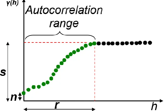
The typical shape of a () function is illustrated in Figure 2. Example functions suitable

181

to model isotropic homogeneous variogram models, but many more exist in literature, 182 are: 183 184 2 2 0 0

( ) Gaussian model

n s 1-exp -3 0 r

0 0

( ) Exponential model

n s 1-exp -3 0 r

0 0

( ) n s 1-exp -3 0 r Spherical model r

n s r

h h h h h h h h h h h h h         _{ }         _{ }        _    _     _{  }                          (4) 185 186

where s, n, r are a sill, nugget, and range, respectively. These three parameters 187

characterize all variogram models (Figure 2). Nugget (n) is a non-zero limit 188

representing a discontinuity in a variogram origin. The nugget represents the pure white 189

noise included in the random error. Sill (s) quantifies the error dispersion at infinite 190

distance, i.e. global correlated and uncorrelated measurement noise. Range (r) is a 191

measure of the distance up to which the measurement noise is significantly correlated. 192

Supposing the variogram error model and its parameters are known, having defined 193

a set of locations 𝐱, the Σmatrix can be built as 194

195

𝛴𝑖𝑗 = 𝑠 − 𝛾(𝐱𝑖, 𝐱𝑗) (5)

196 197

Once the Σmatrix is known any multi-normal random number generator can be applied 198

to generate the 𝜀𝑧𝑖 term at the 𝐱𝑖 location.

199 200

201

Figure 2: Illustration of variogram function and its s, r, n parameters. 202

6 2.2 Estimation of the variogram parameters for the simulation

204

The variogram model and its parameters need experimental identifications and 205

evaluations. From experimental data, a least-square method is usually adopted to fit the

206

empirical model of the variogram. Given a set of observations 𝑍(𝐱𝑖) (e.g. a single scan

207

of a surface by 3DM), the value of the variogram at distance h can be estimated as 208

209

𝛾̂(ℎ) =_2|𝑁(ℎ)|1 ∑_𝑁(ℎ)(𝑍(𝐱_𝑖) − 𝑍(𝐱_𝑗))2 (6) 210

𝑁(ℎ) = {(𝐱𝑖, 𝐱𝑗)|‖𝐱𝑖− 𝐱𝑗‖ = ℎ} (7)

211 212

In the specific case of 3DM, as the points are locate on an evenly spaced grid, the 213

possible values of h are well defined, so there are a series of well-defined values of 214

𝛾̂(ℎ). The 𝛾̂(ℎ) are then fitted, considering different variogram models. Based on R2 215

of the least-square fitting, the best-fitted variogram model is selected, and then, the n, 216

s, and r parameters are estimated. 217

The least square estimation of the s, n, and r parameters is in general applicable to a 218

single sampled surface. It is then evident that the resulting parameters will be specific 219

for the particular condition at which the scan has been conducted, e.g. material type. To 220

have parameters that can be applied in a larger variety of conditions, we must modify 221

them in order to take into account other uncertainty contributors. While the estimate of 222

the nugget and the range can be properly estimated on a single scan, the sill, being 223

representative of the overall variability of the measurement noise (correlated and 224

uncorrelated), should include all the uncertainty contributors, and not only those from 225

the condition at which it has been characterized so far. Hence, the parameter s resulting 226

from the least square fitting shall be combined with other error sources before the 227

simulation, according to the formula: 228

229

2 2

s_sim  s 



230 231

where sis the sill originally obtained from the fitted model of the variogram and si

232

is the contribution related with the ith source of error. The estimate of the 𝑠_𝑖 terms 233

require a deep analysis of the specific uncertainty sources affecting a particular 3D 234

microscope, and an extensive experimental investigation of them. O nce the 235

contributors are known, their value can be extended to any future measurement. 236

237

3. Case study: the uncertainty estimation for a Focus Variation Microscope

238 239

Focus variation microscopy (FVM) is considered in this study as an example of 3DM. 240

The FVM instrument used to demonstrate the proposed simulation approach is a 4th

241

generation FVM instrument by Alicona Imaging GmbH. 242

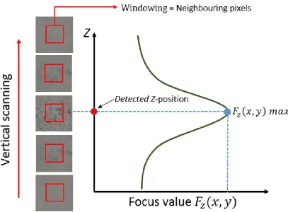
A FVM works based on the local focus condition of a stack of images taken at 243

different distances from the measured surface to the FVM objective lens. The FVM 244

working principle is as follows (see Figure 3): first, a stack of images is taken over a 245

specified range of z-level (the distance from the measured surface to the scanning 246

objective lens); the stack image acquisition is usually obtained by mechanically moving 247

the objective lens of the FVM. For each z-level and for each pixel of the related stacked 248

images, a focus value 𝐹𝑧(𝑥, 𝑦), which is a contrast of a pixel with respect to its

249

7 higher the focus value is. For each pixel a mathematical fitting procedure is applied to 251

the calculated focus values at each level, and the detected z-coordinate of a point is 252

determined corresponding to the z-level with the highest 𝐹_𝑧(𝑥, 𝑦) [15]. 253

One fundamental advantage of a FVM instrument compared to other optical 254

microscopy is its large working volume and its long working distance of the objective 255

lens. This fundamental advantage provides the possibility of measuring the geometrical 256

properties of a part. 257

The FV values calculated for each (i,j) pixel locations are obtained by comparing its 258

contrast with respect to the intensity of its neighbor pixels. 259

260

261

Figure 3: FVM working principle by calculating a focus value inside a windowing 262

area. 263

264

3.1. Estimation of the variogram parameters 265

Different materials can be characterized by different variograms. In this study, we 266

consider calibrated plates of aluminum (Al), stainless steel (SS), and titanium (Ti) for 267

the variogram characterizations. It is worth to note that the variogram characterization 268

data need to be obtained from a real surface in order to take into account the physical 269

properties of the real measured surface, e.g. a roughness effect, local slope effect, 270

reflectance effect, measurement angle effect and speckle noise effect of the surface to 271

be included into the simulation process. Hence the variogram model takes into account 272

the material type as uncertainty source. The variogram data from the actual surface 273

measurements from the mentioned three materials will be used for uncertainty 274

estimation with industrial case studies (section 4). 275

The variogram characterization, required to estimate the degree of a spatial 276

correlation among points, is a fast procedure. The procedure only takes one single 277

measurement with a single image field of a surface to be measured. It is worth noting 278

8 sufficient to characterize the variogram because in an empirical variogram estimate 280

every couple of points counts as a variance estimate replica. 281

The flatness of the three materials was calibrated by means of a traceable CMM with 282

E0,MPE=2+L/300 µm. Methods selected for the calibration are position and

multi-283

measurement strategies. A total of four different positions for the part were considered 284

during the calibration of the plates. For each position, five measurements were repeated. 285

By this method, an uncertainty contribution of the volumetric error of the CMM is also 286

taken into account in the total calibration uncertainty. The results of the flatness 287

calibration and their uncertainty are (notation is based on GUM [4]): aluminum = 288

25.1(8) µm, stainless steel = 4.8(1) µm, and titanium = 4.1(2) µm. 289

To yield the data on which to define the variogram models, the plates were measured 290

having the optical axis of the FVM approximately perpendicular to the plate itself, using 291

the scan parameters in Table 1. The empirical variogram was then evaluated on these 292

scanned surfaces. The variogram models in Eq. 4 are least-square fitted and the 293

parameters s, n, and r are calculated. The model is selected based on the highest R2 294

value of the data fitting. Table 2 presents the selected variogram models and their R2

295

value for the considered three materials (Al, SS, Ti). Detailed variogram 296

characterizations can be found in [17]. The nugget effect has been indicated equal to 0 297

because its value did not differ significantly from 0. This indicates a very strong 298

statistical correlation among measurement errors at short distances, which is due to the 299

FVM measurement principle based on a focus value calculated over a small patch of 300

pixels. 301

Regarding the vertical and lateral resolution, they are set following the default values 302

proposed by the instrument manufacturer with a 5× objective lens. It is worth noting 303

that the selected lateral resolution is larger than the pixel size of the instrument. For the 304

5× objective lens, the pixel size is 1.76 µm. But, the actual resolution (the smallest 305

distance between two features that can be resolved) will be larger than the pixel size 306

due to the working principle of the instrument. As the measuring principle of the 307

instrument needs the consideration of a patch of pixels around the considered point to 308

calculate the focus measure that defines the z-level of the point, the effective resolution 309

is reduced by the averaging effect of the focus measure estimated on the patch (see 310

figure 3). 311

Table 1 Measurement parameter for Al, SS, and Ti materials. 312

Material Exposure

time [µs]

Contrast Vertical

Resolution [µm]

Lateral Resolution [µm]

Aluminum 114.4 1.33 0.4 7.82

Stainless steel 116.4 1 0.4 7.82

Titanium 224 1 0.4 7.82

313

Table 2 Selected variogram model for Al, SS and Ti. 314

Material Variogram

model R

2 _{s [µm] n [µm] r [µm]}

Aluminum (Al) Exponential 0.56 31 0 114 Stainless steel (SS) Exponential 0.78 2.8 0 56

Titanium (Ti) Gaussian 0.71 3.9 0 18

315

3.2. Estimation of the contributors to the sill value for the simulation 316

An extensive experimental campaign was carried out to estimate the various 𝑠_𝑖 terms 317

involved in FVM measurements. Therefore, the physical aspects of a FVM 318

9 A FVM uses a sensor to take a series of images at different distances from a surface. 320

A focus value is then calculated and a height is associate to each pixel. In case, stitching 321

can be applied to increase the size of the scan. This process is prone to a lot of 322

uncertainty sources that cannot be considered by the experiment proposed in section 323

3.1. Therefore, more uncertainty sources are estimated. Figure 4 schematically depicts 324

the main uncertainty contributors in FVM measurements. 325

326

327

Figure 4: Diagram of the uncertainty contributors in FVM measurements [17]. 328

329

An extensive experimental campaign has been conducted to study and quantify the 330

effect of the mentioned factors and to include them into the simulation parameters. The 331

three materials already mentioned were considered: aluminum (Al, specular surface), 332

stainless steel (SS, lambertian surface), and titanium (Ti, lambertian surface). The 333

numbers of points produced by a FVM measurement ranges from ~1 to ~4 million 3D 334

spatial points. The analysis of variance (ANOVA) has been used to determine the 335

significance of the factors. 336

Outliers were removed from the obtained datasets before measurement results could 337

be extracted. This procedure is important since a large data point set is obtained from a 338

single measurement cycle and outlying points among these points (points presenting a 339

very large algebraic deviation compared to other points in the scan) could reduce the 340

accuracy of the measurement result. A simple outliers removal procedure has been 341

applied, i.e. points having a deviation greater than 3σ from the fitting plane or cylinder 342

of data points (depending on measured form) were removed, where σ is the sample 343

standard deviation of all point deviations (residuals), that are distances from points to 344

the fitted geometry. 345

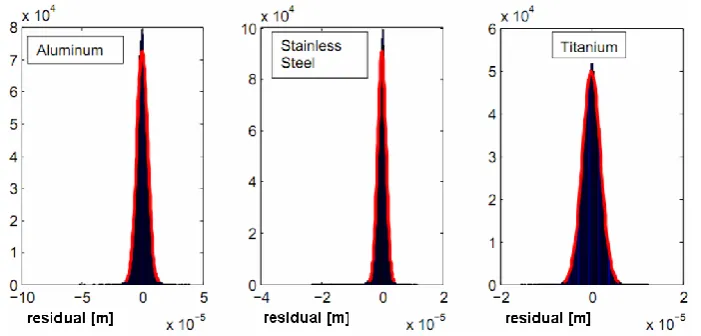
A Shapiro-Wilk test, applied to the residuals (errors) of measured points, proved 346

normality of the deviations with p-value around 0.8 for all the datasets. Figure 5 shows 347

the histogram of the deviations (residuals) of points to the fitted plane for the three 348

materials. The red line is the fitted Gaussian density function. The standard deviation 349

(σ) of the residuals is presented in Table 3. 350

In this uncertainty characterization studies, the standard deviation σ of measurement 351

residuals due to different parameters and measurement conditions is considered as 352

parameter characterizing the impact or effect on the measurement uncertainty. The 353

measurement residuals are σ of point deviations (a point distance error) to a fitted 354

geometry, e.g. a plane, sphere and cylinder. 355

356

Measurement Uncertainty

Machine (Instrument Parameters)

Exposure time Contrast Vertical Resolution

Lateral Resolution

-Materials (Part shape &Illumination)

PeakValley shape

Material types

Illumination types

-Methods (Procedure)

Stitching

Part orientation

Magnification

-Environment

Drift

-10 357

Figure 5: Histogram of residual from a fitted plane for the Aluminum, Stainless 358

steel and Titanium materials. 359

360

Table 3 Standard deviation of residuals for the three materials. 361

Material σ[µm]

Aluminum (Al) 4.49 Stainless steel (SS) 1.37 Titanium (Ti) 2.00

362

3.2.1 Influence of ambient light and different magnification lenses 363

364

A randomly structured surface of a polymeric injection-molded part was used to 365

evaluate this contribution. The polymeric surface is considered because it has a high 366

surface diffusivity and low roughness < 200 nm. Therefore, the surface is smooth and 367

good to estimate the measurement repeatability in the study and to understand the effect 368

of ambient light in a FVM measurement. 369

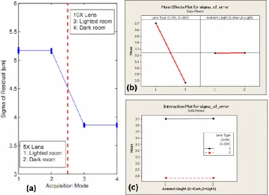
Measurements were carried out at 5× and 10× magnifications, both with the ambient 370

light switched on or off. Numbers of 20 repetitions were carried out with around ~1 371

million points in each measurement repetition. Figure 6a plots the sigma of the residuals 372

obtained by measuring with different lens types and ambient illuminations. In this 373

figure, there are two sections. The left section presents results obtained using the 5× 374

lens in an illuminated or dark room, while the right section presents the result obtained 375

using the 10× lens. The main effect and interaction plot between the objective lenses 376

and ambient light are shown in figure 6b and 6c, respectively. 377

From the obtained results, it seems that no influence of the ambient light is present. 378

The different magnification is significant instead. The σ of the residuals at 10× reduces 379

to 2.8 µm from the 3.7 µm obtained at 5×. The interaction between magnifications and 380

ambient light is found to be not statistically significant. The range of σ for the lighted 381

and dark room is around 0.01 µm. Meanwhile for difference lenses (magnification 382

11 384

Figure 6: (a) Plot of sigma of residual obtained by different lenses and ambient 385

light, (b) Main effect and (c) Interaction plot between the two factors. 386

387

3.2.2 Influence of different types of illumination 388

389

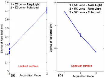
In this study, two materials were used, aluminum (specular) and random-structured 390

polymer (lambertian) [18]. A 5× magnification was used. For each sample, 20 391

measurements were carried out (~1 million points each). The FVM instrument is 392

equipped with three illuminators: axial-light, ring-light and polarized-light. From the 393

analysis, different illuminations significantly affect σ. 394

From figure 7, for the aluminum surface (specular) the difference of σ from ring-light 395

to polarized light reduces by about 0.6 µm, while for the polymer one, it increases by 396

about 0.45 µm. Furthermore, the σ has inverse behavior when moving from specular to 397

lambertian surface. Note that the plot of σ for the lambertian surface is only for ring 398

light and polarized light since the surface cannot be captured with the axial light. The 399

range of σ the different types of illumination with lambert surface is around 0.5 µm and 400

with specular surface is around 1 µm. 401

12 403

Figure 7: Effect of different illuminations for (a) Lambert surface and (b) Specular 404

surface. 405

406

3.2.3 Influence of part orientations (surface slopes) 407

408

The three flat samples made respectively of aluminum, stainless steel, and titanium 409

with the addition of coated steel (lambertian) and steel (specular) were used. The 410

measurements were carried out for four different positions and steepness/slope 411

orientations (00, 50, 100, 150). There are four position types which are combinations of 412

two types of sample placement directions (along x-axis/horizontal or along y-413

axis/vertical) and two types of rotation directions (clockwise or anti-clockwise). Five 414

measurement repetitions were carried out using the 5× objective lens, so in total 80 415

measurements were carried out for each material. 416

From the analysis, it is found that these factors significantly affect the σ. The range 417

of σ for different types of measurement for aluminum, stainless steel and titanium varies 418

around 2.5 µm, 2 µm and 1 µm, respectively. Figure 8 shows the plot of σ for each 419

experiment as well as the measurement process (position and tilt/orientation direction). 420

Figure 8 shows the plot of σ for different positions and different degrees of steepness 421

(orientation). Note that for steel there are no data when the steepness is higher than 50 422

due to the specular reflectivity of the steel material, which causes the measurement to 423

fail. The range of σ for the part orientation is around 3 µm considering the highest range 424

value observed is for aluminum-ring light (figure 8 right: blue line). 425

13 428

Figure 8: Results of σ for part orientation experiments. 429

430

3.2.4 Influence of peak-valley shape measurements 431

432

A machined part having peak and valley features (saw-tooth), made of glazed 433

aluminum with grey color (lambertian), has been used. The edge of the machined part 434

(either peak or valley) was measured 50 times. Each measurement generated about 435

45000 points. The σ in this case is the standard deviation of the distance of a point to a 436

fitted 3D line representing an edge feature. The results show a statistically significant 437

difference of σ between the two different shapes. The σ of peak measurement is lower 438

by about 1.5 µm with respect to the valley one. The peak-valley measurement and the 439

obtained σ are shown in figure 9. The range of σ for the peak-valley shape contributor 440

is around 2.2 µm (by neglecting some outliers points in figure 9). 441

442

14 3.2.5 Stitching/no-stitching measurements

444 445

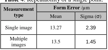
Two types of sphere measurement were carried out: a single image (no-stitching) and 446

four multiple images measurements. The measured part is an ISO 3290-1 steel sphere 447

[19]. Numbers of 50 measurement repetitions were carried out generating ~750000 448

points per scan for a single image measurements and ~ 3250000 points for multiple 449

ones. Table 4 provides details of the results of a point repeatability. The point is derived 450

from the center of a fitted sphere to the obtained points. 451

The results show that the σ, in x-, y- and z-direction, of measurements by stitching are 452

two times lower than the one without stitching. Hence, by stitching procedure, there is 453

an averaging effect to the calculated position of the obtained points which suppresses 454

part of the random error. Form errors in table 4 are the minimum distance between two 455

concentric spheres covering all the obtained points. The range of σ for the stitching of 456

multiple image measurements is around 0.9 µm. 457

458

Table 4: Repeatability of a single point. 459

Measurement type

Form Error /µm

Mean Sigma (σ)

Single image 13.27 2.39

Multiple

images 13.5 1.45

460

3.2.6 Influence of measurement parameters 461

462

There are four main parameters of an FVM measurement: exposure time, contrast, 463

vertical and lateral resolutions. These factors can be controlled by the user before the 464

measurement is carried out. A flat sample made of titanium was used for the study. 465

There are four considered levels for lateral and vertical resolution factors and three 466

levels for exposure time and contrast factors. The range of the lateral and vertical 467

resolutions is based on the resolution limit of a 5× objective lens used for the 468

experiments. Conversely, the selected range for exposure time and contrast were based 469

on the range in which a good scan of the surface can be obtained. Table 5 and Table 6 470

present details of the lateral-vertical study and brightness-exposure time study, 471

respectively. 472

From the analysis of experiment for the lateral and vertical resolution factors, it is 473

found that only the lateral resolution is significant. As it can be seen in figure 10, the 474

lower the lateral resolution is, the smaller the σ is. Decimation of points for bigger 475

lateral resolution could be the reason for the reduction of noise since there is an 476

averaging effect in data processing algorithms. There is no interaction effect between 477

lateral and vertical resolutions as it can be observed in figure 11. 478

These results can be applied in practice for geometric measurement, in particular form 479

measurement. As stated by Evans [11] optical instruments have considerably larger 480

noise compared to contact ones. As form measurement is very sensitive to noise a larger 481

lateral resolution is preferable to suppress measurement noise. The range of σ for the 482

lateral and vertical resolution are around 3 µm and 0.01 µm. 483

15

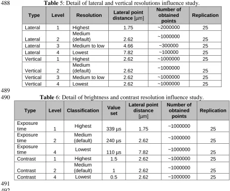
Table 5: Detail of lateral and vertical resolutions influence study. 488

Type Level Resolution Lateral point distance [µm]

Number of obtained

points

Replication

Lateral 1 Highest 1.75 ~2000000 25

Lateral 2

Medium

(default) 2.62 ~1000000 25

Lateral 3 Medium to low 4.66 ~300000 25

Lateral 4 Lowest 7.82 ~100000 25

Vertical 1 Highest 2.62 ~1000000 25

Vertical 2

Medium

(default) 2.62 ~1000000 25

Vertical 3 Medium to low 2.62 ~1000000 25

Vertical 4 Lowest 2.62 ~1000000 25

489

Table 6: Detail of brightness and contrast resolution influence study. 490

Type Level Classification Value set

Lateral point distance

[µm]

Number of obtained

points

Replication

Exposure

time 1 Highest 339 µs 1.75 ~1000000 25

Exposure

time 2

Medium

(default) 240 µs 2.62 ~1000000 25

Exposure

time 4 Lowest 110 µs 7.82 ~1000000 25

Contrast 1 Highest 1.5 2.62 ~1000000 25

Contrast 2

Medium

(default) 1 2.62 ~1000000 25

Contrast 4 Lowest 0.5 2.62 ~1000000 25

16 493

Figure 10: Effect of lateral and vertical resolutions. 494

495

496

Figure 11: Interaction plot between lateral and vertical resolutions. 497

498

Exposure time (brightness) and contrast effects were then considered. From this 499

analysis, it is shown that exposure time and contrast are significantly affecting the 500

sigma of residual σ. Figure 12 shows that σ decreases when both exposure time and 501

17 found significant (figure 13). The range of σ for the contrast and exposure time settings 503

are 0.2 µm and 0.3 µm, respectively. 504

505

506

Figure 12: Effect of different levels of exposure time and contrast. 507

508

509

Figure 13: Interaction plot between the exposure time and contrast. 510

511

3.2.7 Long measurement (drift) behaviors 512

513

The variation of σ due to long measurement, both with and without stitching, has been 514

18 components drift can be a relevant uncertainty source.The titanium flat sample has been 516

used for measurements without stitching. 517

Measurements without stitching do not involve stage movements. Instead, for 518

measurements with stitching from four images, an ISO 3290-1 steel sphere was used. 519

The purpose of this type of measurements is to observe the behavior of the instrument 520

in continuous measurement involving stage movements. Both types of measurements 521

were carried out continuously without operator interventions. Thanks to a scripting 522

ability of the instrument, this continuous measurement can be automatically run by the 523

FVM instrument. The measurement used a 5× magnification lens with default lateral 524

and vertical resolutions. 525

For non-stitching measurements, a total of 30 runs (~1 million points obtained for 526

each measurement run) were carried out with a time span of around five hours. Sigma 527

of residual σ and flatness are calculated for each measurement. Range of σ for this 528

period of time is 0.0067 µm. Results of flatness measurements show a decreasing trend 529

up to the 10th measurement sequence. The flatness interval (95%) for the first 100 530

minutes of measurement is 1.25 µm. After this 100 minutes period, the interval becomes 531

0.62 µm. 532

To represent a systematic error, measurements of distances from i-th plane to a 533

reference plane (plane fitted from the first measurement) were conducted as can be seen 534

from figure 14. In this figure, the systematic error representation is defined as the 535

distance from the center point of the fitted plane of measurement i to the reference plane 536

(plane fitted from the points of the first measurement). They show that the variation 537

range (95%) of the distance during the first 19 measurements (the first 190 min.) is 0.16 538

µm, while after this period, it increases to 2.72 µm. Note that the value is shifted one 539

position to the left, since the 1st measurement is not included. Starting from the 20th 540

measurement, juggling phenomena of the measured distance to the reference plane of 541

the flatness can be observed. These results are presented in figure 15. 542

543

544

Figure 14: Illustration of distance to reference plane. 545

19 547

Figure 15: Long continuous measurement behaviors by plane measurements (without 548

stitching). 549

550

Measurements of a sphere with stitching were carried out for 45 runs (~3 millions of 551

points for each measurement run) which correspond to a six hour period. Parameters 552

calculated from the measurement include sigma of the residuals σ, the distance of two 553

consecutive centers and the sphere form error. The sigma of the residuals is used to 554

represent a random error. For a systematic error representation, distances between two 555

consecutive centers are calculated. A stable variation was observed during the first 40 556

measurements (the first 320 minutes). A shifting is observed for σ after 320 minutes is 557

around 3 µm and for form error is about 40 µm, while the shift between the center 558

distances is about 25 µm. Figure 16 presents the plot of the measurement drift behavior 559

for this type of measurement. The range of σ for the drift is around 2 µm. 560

20 563

Figure 16: Long continuous measurement behavior by sphere measurements (with 564

stitching). 565

566

3.3 Summary of the contributions 567

568

Finally, to summarize all the results from the uncertainty characterisation study, table 569

7 shows the range of the variation of σ for all the considered factors (worst-case 570

scenarios). These values, that are considered relevant in each measurement task, are the 571

𝑠𝑖 values included in the sill 𝑠𝑠𝑖𝑚 parameter used in the simulation model (equation 5).

572 573

Table 7: Summary of the influence of the factors. 574

Factor Effect σ [µm]

Peak-Valley shape Significant 2.2

Illumination type with lambert surface Significant 0.5 Illumination type with specular surface Significant 1

Lateral Resolution Significant 3

Vertical Resolution Not Significant 0.01

Exposure time Significant 0.3

Contrast Significant 0.2

Stitching Significant 0.9

Magnification Significant 1.3

Part orientation Significant 3

Drift Significant 2

Ambient light Not Significant 0.01

4. Validation

575

The ISO/TS 15530-4 standard [10] is the basis for the application and validation to 576

guarantee the traceability of a simulation-based uncertainty estimation in coordinate 577

metrology. As there are several deeply different coordinate measuring systems, the 578

ISO/TS 15530-4 standard cannot define a general methodology for simulating the 579

measurement and stating the uncertainty based on the simulation results. Instead, the 580

ISO/TS 15530-4 standard defines the general requirements for the simulation, and the 581

21 The validation according to the ISO/TS 15530-4 standard includes both the 583

mathematical model and the model parameters. The ISO/TS 15530-4 states that: 584

585

“Performing a number of measurements on calibrated objects, the coverage of the 586

uncertainty ranges is checked. The plausibility criterion should be satisfied for an 587

appropriate percentage of the time (95% for k = 2); this criterion is that a statement of 588

uncertainty is plausible if: |𝑦 − 𝑦_𝑐𝑎𝑙|/√𝑈_𝑐𝑎𝑙2 + 𝑈2 ≤ 1”. 589

590

In this method, one should then calculate a En value for each measurement run. En is 591

formulated as: 592

593

2 2

cal

n cal

E |yy | / U U (9) 594

595

where y is a measurement result, ycal is the calibrated value of y, Ucal is the expanded

596

calibration uncertainty, and U is the expanded uncertainty obtained by simulation. If 597

the expansion factor k is equal to 2, a good agreement can be concluded if 598

approximately 95% of total measurements runs are characterized by En< 1. 599

Several case studies of geometric measurements are considered to validate the 600

proposed simulation method; they include form (flatness measurements) and size 601

measurements (diameter and height measurements). More complicated case studies can 602

be found in [17]. It is worth to note that although the components are not a micro-sized 603

component, the portion of features of the measured component and tolerances are at 604

micro-scale [1, 2]. In the case study, the variogram model, used for uncertainty 605

estimations by the proposed simulation, are selected based on the type of the material 606

of the cased study considered. 607

608

4.1 Flatness measurement 609

610

The three calibrated samples originally adopted for the definition of the variogram 611

models were considered (see §3.1). The simulation is applied to points obtained from a 612

real measurement. Therefore, feature form deviation of the part is already included [20]. 613

Figure 17 qualitatively shows that a variogram based simulation yields better results 614

compared to a simulation of uncorrelated points. The red line shows the simulation 615

result if the variogram model is applied: it is clear that it is close to the original data. 616

Instead, if the noise is simulated as pure white noise with a standard deviation equal to 617

the sill s of the variogram, the simulation result is far from the original data (green 618

points). 619

Numbers of 100 flatness measurement runs were carried out by changing the part 620

orientation (approximately perpendicular to the optical axis, 5° _{tilted clockwise and}

621

anticlockwise) to represent an orientation error when placing the part. The measurement 622

parameters used followed those shown in Table 1 for each material type and orientation. 623

To evaluate the uncertainty, 500 simulation runs were carried out. The sill s parameter 624

of the simulation was modified according to Eq. (5) to consider the influence of the 625

various uncertainty factors in the real measurement situation of the flatness 626

measurement. Figure 18a shows results of the flatness measurements. It is worth noting 627

that the flatness is based on a min-max fitting. This kind of fitting in general generates 628

a non-Gaussian distribution of the measurement results. 629

22 The flatness samples were calibrated on a traceable tactile-CMM with E0;MPE = 2 +

631

L/300 µm where L is the measured length in mm (the CMM is periodically performance 632

verified). The calibrations follows a multiple-measurements strategy that vary the 633

position and orientation of the samples during the calibration process to take into 634

account the volumetric error of the traceable tactile-CMM. Calibration results of the 635

flat samples are y = 25.1 µm and _cal Ucal = 1.6 µm for Al, y = 4.8 µm and cal Ucal = 0.2

636

µm for SS, and y = 4.1 µm and _cal Ucal = 0.4 µm for Ti.

637

The estimated U for Al, SS, and Ti are 14.0 µm, 7.7 µm, and 10.1 µm, respectively. 638

From calculation of each Envalue, the fraction of Envalues for which En < 1 for Al, SS, 639

and Ti are 97%, 96%, and 98% respectively (Figure 18b), so the simulator can be 640

considered validated in this case. From figure 18, some portions of En are larger than 641

one. Having some portion of En > 1 suggest that the estimated uncertainty by the 642

proposed simulation is not overestimating the expected uncertainty. Similar explanation 643

for the En values are valid for all other presented case studies in this paper. 644

645 646

647

Figure 17: Plot of original points (blue) superimposed with the simulated points 648

without considering (green) and with considering (red) the correlation among points 649

for aluminum (Al), stainless steel (SS), and titanium (Ti). 650

23 652

Figure 18: Plot of (a) histogram of the flatness value and (b) Envalues for the flatness 653

measurement of Al, SS, and Ti. 654

655

4.2. Commercial micro-wire measurements 656

The measurement of a diameter (a dimensional characteristic) is presented in this 657

case. An industrial micro steel wire with diameter of 310±2 µm was measured (Figure 658

19). The wire is used as a plug-gage to measure the nozzle diameter of a water jet 659

machine. Since the part is a commercial plug-gage, ycaland Ucalare based on the part’s

660

nominal specifications. The ycal is considered to be equal to 310 µm. The Ucal of the

661

plug-gage diameter is estimated as a type B uncertainty and is assumed to have a 662

rectangular distribution. Hence, Ucal is equal to 2.31 µm.

663

Before running the simulation, the procedure, explained in Section 2, to determine 664

the variogram model was carried out for steel since the variogram model of the steel 665

material used in this case study has not yet been determined. The selected variogram 666

model is a Gaussian one with s, n, and r parameters equal to 34.4 µm, 0 µm, and 14.8 667

µmm respectively. The estimated U is 5.6 µm obtained from 500 simulation runs 𝑦. A 668

total of 85 measurement runs 𝑦 were carried out with the following measurement 669

parameters: 193.2 ms (exposure time), 0.44 (contrast), 0.6 µm (vertical res.) and 3.9 670

µm (lateral res.) by using 10× objective lens. From the En calculation, a total of 98 % 671

values have En < 1, thus ensuring validation. The histogram of the measurement results 672

𝑦 and the En calculation for each measurement are shown in figure 20. In figure 20 673

right, around 2 % of En values are more than one. 674

24 676

Figure 19: The micro-wire. 677

678

Figure 20: (a) Histogram of the diameter measurement results and (b) En values for 679

the diameter measurement validation. 680

681

4.3. Step-height measurements of a slot-milled steel component 682

683

A measurement of the step-height of a slot-milled part is presented in this study. The 684

part was made of a steel material by using a precision micro-milling machine. The part, 685

the slot height definition and an example of the measured surface are shown in figure 686

21. Measurement parameters for the slot step-height measurement are exposure time = 687

88.32 µs, contrast = 0.2, lateral resolution = 7.83 µm and vertical resolution = 0.4 µm 688

by using a 5× objective lens. 689

The results of a calibration process using a traceable tactile-CMM are y = 698.7 _cal 690

µm and expanded uncertainty Ucal = 0.25 µm. Total of 100 measurements runs 𝑦 was

691

carried out. From around 500 simulations runs to estimate the uncertainty of the slot 692

measurement, an expanded estimated uncertainty U is obtained as 0.45 µm. From a 693

total of 100 measurement runs 𝑦, 93% (almost 95%) of En values are less than 1, hence 694

25 histogram of the measurement results and the En value calculation for each 696

measurement. 697

698

699

Figure 21: The measured slot and its obtained surface. 700

701

702

Figure 22: (a) Histogram of the height measurement results and (b) En values for the 703

slot step-height measurement validation. 704

5. Conclusions

705

This paper presents a proposal of a simulation-based approach to estimate the task-706

specific measurement uncertainty of a 3DM performing geometric inspections. A case 707

study regarding FVM is proposed. The case study is validated according to the ISO/TS 708

15530-4 standard. The method considers the correlation among points obtained by the 709

optical instrument since correlation naturally occurs among points measured 710

sequentially or continuously. Variogram models are determined for each material to 711

represent the property of correlations among points. In general, the correct type of 712

variogram (Gaussian, exponential, spherical, etc.) is defined based on the gathered 713

26 we developed and validated in a case study. The proposed approach can be applied to 715

other type of 3DM instruments and can be implemented and integrated into instruments 716

software system as a module. 717

Extensive uncertainty characterization has been carried out to identify and quantify 718

the uncertainty sources and incorporate them into the simulation parameters. The 719

validation is carried out with industrial case studies and the results show that the 720

simulated uncertainties have a good agreement with the real measurement. 721

The proposed simulation approached can be summarised as follows: 722

1. Define the variogram model and quantify the s, n and r parameters for each 723

material type. This step is carried out once for every different material. 724

2. Experimentally evaluate the additional uncertainty sources not considered in the 725

variogram, but influencing the measurement result. The uncertainty sources 726

quantification is carried out once for each type of instrument. 727

3. Measure the part to inspect, and compute the measured value 𝑦. 728

4. Having modified the value of s considering the additional sources of uncertainty, 729

apply the variogram model to generate an adequate number of simulation runs 730

and the related perturbed clouds of points, compute the simulated measured values 731

and, based on these values, estimate the expanded uncertainty U. 732

5. State the measurement result 𝑦 ± 𝑈. 733

Further works include building a database of optimal variograms for various types of 734

materials and applying the proposed method to estimate task-specific uncertainty for 735

surface texture measurements. 736

737

Acknowledgements

738 739

Financial support to this work has been provided as part of the project REMS - Rete 740

Lombarda di Eccellenza per la Meccanica Strumentale e Laboratorio Esteso, funded by 741

Lombardy Region (Italy), CUP: D81J10000220005 and AMala – Advanced 742

Manufacturing Laboratory, funded by Politecnico di Milano (Italy), CUP: 743

D46D13000540005. 744

Acknowledgment is due to the Recruitment Program of High-end Foreign Experts of 745

the Chinese State Administration of Foreign Experts Affairs. 746

747

References

748

[1] L. Alting, F. Kimura, H. Hansen, G. Bissacco, Micro engineering, CIRP Annals 749

- Manufacturing Technology 52 (2) (2003) 635–657. doi:10.1016/S0007-750

8506(07)60208-X. 751

[2] H. Hansen, K. Carneiro, H. Haitjema, L. De Chiffre, Dimensional micro and 752

nano metrology, CIRP Annals - Manufacturing Technology 55 (2) (2006) 721–743. 753

doi:10.1016/j.cirp.2006.10.005. 754

[3] ISO/IEC, ISO/IEC GUIDE 99:2007(E/F): International vocabulary of 755

metrology - basic and general concepts and associated terms (VIM) (2007). 756

[4] G. Moroni, S. Petrò, W. Syam, Four-axis micro measuring systems 757

performance verification, CIRP Annals - Manufacturing Technology 63 (1) (2014) 758

485–488. doi:10.1016/j.cirp.2014.03.033. 759

[5] G. Moroni, W. Syam, S. Petrò, Performance verification of a 4-axis focus 760

variation co-ordinate measuring system, IEEE Transactions on Instrumentation and 761

Measurement 66 (1) (2017) 113–121. doi:10.1109/TIM.2016.2614753. 762

[6] ISO/IEC, ISO/IEC GUIDE 98-3: Uncertainty of measurement - Part 3: Guide 763

27 [7] R. Wilhelm, R. Hocken, H. Schwenke, Task specific uncertainty in coordinate 765

measurement, CIRP Annals - Manufacturing Technology 50 (2) (2001) 553–563. 766

doi:10.1016/S0007-8506(07)62995-3. 767

[8] G. Moroni, S. Petrò, Optimal inspection strategy planning for geometric 768

tolerance verification, Precision Engineering 38 (1) (2014) 71–81. 769

doi:10.1016/j.precisioneng.2013.07.006. 770

[9] International Organization for Standardization, ISO 15530-3: Geometrical 771

Product Specifications (GPS) – Coordinate measuring machines (CMM): Technique 772

for determining the uncertainty of measurement – Part 3: Use of calibrated workpieces 773

or standards (2011). 774

[10] International Organization for Standardization, ISO/TS 15530-4: Geometrical 775

Product Specifications (GPS) - Coordinate measuring machines (CMM): Technique for 776

determining the uncertainty of measurement - Part 4: Evaluating task-specific 777

measurement uncertainty using simulation - First Edition (Jun. 2008). 778

[11] C. Evans, Uncertainty evaluation for measurements of peak-to-valley surface 779

form errors, CIRP Annals - Manufacturing Technology 57 (1) (2008) 509–512. 780

doi:10.1016/j.cirp.2008.03.084. 781

[12] J.-P. Kruth, N. Van Gestel, P. Bleys, F. Welkenhuyzen, Uncertainty 782

determination for cmms by monte carlo simulation integrating feature form deviations, 783

CIRP Annals - Manufacturing Technology 58 (1) (2009) 463–466. 784

doi:10.1016/j.cirp.2009.03.028. 785

[13] C. Cheung, M. Ren, L. Kong, D. Whitehouse, Modelling and analysis of 786

uncertainty in the form characterization of ultra-precision freeform surfaces on 787

coordinate measuring machines, CIRP Annals - Manufacturing Technology 63 (1) 788

(2014) 481–484. doi:10.1016/j.cirp.2014.03.032. 789

[14] E. Trapet, F. Waeldele, The virtual CMM concept, in: P. Ciarlini, M. Cox, 790

F. Pavese, D. Richter (Eds.), Advanced Mathematical Tools, II, World Conference 791

Scientific, Singapore, 1996, pp. 238–247. 792

[15] R. Leach (Ed.), Optical Measurement of Surface Topography, Springer-Verlag, 793

Berlin, Germany, 2011. doi:10.1007/978-3-642-12012-1. 794

[16] N. A. C. Cressie, Statistics for Spatial Data, 1st Edition, Wiley-Interscience, 795

New York, 1993. 796

[17] W. P. Syam, www.politesi.polimi.it/handle/10589/100382Uncertainty 797

evaluation and performance verification of a 3d geometric focus variation 798

measurement, Ph.D. thesis, Politecnico di Milano, Milan, Italy (2015). 799

www.politesi.polimi.it/handle/10589/100382 800

[18] D. A. Forsyth, J. Ponce,

801

https://books.google.it/books?id=gM63QQAACAAJComputer Vision: A Modern 802

Approach, Always learning, Pearson, 2012. https://books.google.it/-803

books?id=gM63QQAACAAJ 804

[19] International Organization for Standardization, ISO 3290-1: Rolling bearings – 805

Balls – Part 1: Steel balls (2014). 806

[20] J. M. Baldwin, K. D. Summerhays, D. A. Campbell, R. P. Henke, Application 807

of simulation software to coordinate measurement uncertainty evaluations, NCSLI 808

Measure 2 (4) (2007) 40–52. doi:10.1080/19315775.2007.11721398. 809