arXiv:1607.07974v2 [stat.ME] 4 Aug 2016
Nonparametric hypothesis testing for equality of means on the simplex
Michail Tsagris
1, Simon Preston
2and Andrew T.A. Wood
21
Department of Computer Science, University of Crete, Herakleion,
Greece, [email protected]
2
School of Mathematical Sciences, University of Nottingham,
Nottingham Park, Nottingham, UK
Abstract
In the context of data that lie on the simplex, we investigate use of empirical and exponential empirical likelihood, and Hotelling and James statistics, to test the null hypothesis of equal pop-ulation means based on two independent samples. We perform an extensive numerical study using data simulated from various distributions on the simplex. The results, taken together with practical considerations regarding implementation, support the use of bootstrap-calibrated James statistic.
Keywords: Compositional data, hypothesis testing, Hotelling test, James test, non parametric, empirical likelihood, bootstrap
1
Introduction
Data that lie on the the simplex
Sd=
(
(x1, ..., xD)T
xi≥0, D
X
i=1
xi= 1
)
, (1)
where d=D−1 are sometimes called compositional data, and they arise in many disciplines, including geology (Aitchison, 1982), economics (Fry et al., 2000), archaeology (Baxter et al., 2005) and political sciences (Rodrigues and Lima, 2009).
We consider two forms of nonparametric likelihood: Empirical likelihood (EL) is a non-parametric likelihood which shares many of the properties of non-parametric likelihoods (see Owen (1988, 1990, 2001); Qin and Lawless (1994)); and Exponential Empirical Likelihood (EEL), due to Efron (1981), who obtained it by exponential tilting. EEL has similar first-order asymp-totic properties to EL but different second-order properties, e.g. in contrast to EL, which is Bartlett correctable (DiCiccio and Romano, 1990), EEL is not Bartlett correctable (Jing, 1995). Zhu et al. (2008) consider a correction to EEL. However, in this paper we focus on higher-order corrections based on bootstrap calibration rather than Bartlett correction of other types of an-alytic correction (see Hall and La Scala, 1990, for discussion of these different approaches, and Li et al., 2011). Some kind of correction is usually needed in practice unless the sample size is large because, as has been shown in many simulation studies in a variety of contexts, EL and EEL likelihood ratio tests without correction do not do a good job of controlling Type I error; usually the actual Type I error is larger than the nominal Type I level. Examples of such simulation studies include Diciccio and Romano (1989), Fisher et al. (1996), Emerson (2009), Amaral and Wood (2010) and Preston and Wood (2010).
Our results show that, without correction, EL and EEL based tests tend to be less accurate, in terms of control of Type I error, than other nonparametric methods, such as nonparametric bootstrap versions of the Hotelling and James statistics. Moreover, as we shall see, when bootstrap calibration is applied to EL and EEL testing, it only brings the performance of EL and EEL in line with, but does not surpass, the performance of bootstrapped Hotelling and James statistics. In view of the challenging computational issue in higher dimensions of finding points in the intersection of the supports of the two sample EL or EEL likelihoods, we conclude that, from a practical point of view, bootstrapped Hotelling and James statistics are preferable to use in the setting of the paper, since they are much easier to implement than, yet achieve control of Type I error and power which is as good as, that of bootstrap-calibrated EL and EEL tests.
The outline of the paper is as follows. In Section 2 we review the test statistics to be studied: parametric and nonparametric bootstrap versions of the Hotelling and James statistics, and EL and EEl statistics with and without bootstrap calibration. In Section 3 we presents the results of an extensive simulation study and we present our conclusions in Section 4.
2
Quadratic tests for two population mean vectors
The two quadratic-form test statistics we will use are the Hotelling statistic and James statistic defined as follows.
2.1 Two-sample equality of mean vector test whenΣΣΣ1 = ΣΣΣ2 (Hotelling test)
If the covariance matrices can be assumed equal, the Hotelling T2 test statistic for two d
-dimensional samples is given by (Mardia et al., 1979)
T2 = (¯x1−x¯2)T
Sp
1
n1
+ 1
n2
−1
where Sp = (n1−1)nS1+1+(n2n−22−1)S2 is the pooled covariance matrix with S1 and S2 being the two
unbiased sample covariance matrices
S1 = 1/(n1−1)
n1
X
i=1
[(x1)i−x¯1] [(x1)i−x¯1]T and
S2 = 1/(n2−1)
n1
X
i=1
[(x2)i−x¯2] [(x2)i−x¯2]T,
where ¯x1 and ¯x2 are the two sample means andn1 and n2 are the two sample sizes. UnderH0
and when the central limit theorem holds true for each population we have that
T2∼ (n1+n2)d n1+n2−d+ 1
Fd,n1+n2−d+1.
2.2 Two-sample equality of mean vector test whenΣΣΣ1 6= ΣΣΣ2 (James test)
James (1954) proposed a test for linear form of hypotheses of the population means when the variances are not known. The test statistic for two d-dimensional samples is
Tu2 = (¯x1−x¯2)T S˜−1(¯x1−x¯2), (3)
where ˜S= ˜S1+ ˜S2 = nS11 +Sn22. James (1954) suggested that the test statistic is to be compared
with 2h(α), a corrected χ2 quantile whose form is
2h(α) =χ2ν,1−a A+Bχ2ν,1−a
,
whereχ2νis a chi-squared random variable withνdegrees of freedom, such thatP
χ2ν ≤χ2ν,1−α
= 1−α and
A = 1 + 1 2d
2
X
i=1
h
trS˜−1S˜ i
i2
ni−1
and
B = 1
p(p+ 2)
1 2 2 X i=1 tr ˜ S−1S˜
i
2
ni−1
+ 1 2 2 X i=1 h
trS˜−1S˜ i
i2
ni−1
,
Krishnamoorthy and Yu (2004) showed that under the multivariate normality assumption for each sample
Tu2∼ νd
ν−d+ 1Fd,ν−d+1 approximately,
where
ν= d+d
2
1
n1
trS˜1S˜−1
2
+trS˜1S˜−1
2
+n1
2
trS˜2S˜−1
2
+trS˜2S˜−1
2. (4)
than two samples, whereas Krishnamoorthy and Yu (2004) calculated the degrees of freedom of theF distribution for the two samples only.
2.3 Empirical likelihood for the two sample case
Jing (1995) and Liu et al. (2008) described the two-sample hypothesis testing using empirical likelihood.
The 2 constraints imposed by empirical likelihood
1
nj nj
X
i=1
n
1 +λλλTj (xji−µµµ)
−1
(xij −µµµ)
o
=0, j= 1,2, (5)
where theλλλjsare Lagrnagian parameters introduced to maximize (7). The probabilities of each
of the j samples have the following form
pji =
1
nj
1 +λλλTj (xji−µµµ)−
1
, (6)
where λλλ1+λλλ2 = 0 is a convenient constraint that can be used. The log-likelihood ratio test
statistic can be written as
Λ =
2
X
j=1
nj
X
i=1
lognjpij =
2
X
j=1
nj(¯xj−µµµ)T Sj(µµµ)−1(¯xj −µµµ) +op(1), (7)
whereSj(µµµ) = nj−nj1Sj+ (¯x−µµµ) (¯x−µµµ)T withSj denoting the sample covariance matrix. The
maximization of (7) is with respect to theλλλjs.
Asymptotically, under H0 Λ ∼χ2d, since S(µµµ) p
→ΣΣΣ, where ΣΣΣ is the population covariance matrix. A proof of the asymptotic distribution of the test statistic when we have more than two samples, both in the univariate and multivariate case, can be found in Owen (2001).
However, asymptotically, this test statistic is the same as the test statistic suggested by James (1954). As mentioned in Section 2.2, James (1954) used a corrected χ2 distribution
whose form in the two sample means cases is given in Section 2.2. Therefore we have strong grounds to suggest James corrected χ2 distribution for calibration of the empirical likelihood test statistic instead of the classical χ2 distribution.
Maximization of (7) with respect to a scalar λ, in the univariate case, is easy since a simple search over an interval is enough. In the multivariate case though, the difficulty increases with the dimensionality. Another important issue we highlight is that empirical likelihood test statistic will not be computed ifµµµlies within the convex hull of the data Emerson (2009). This issue becomes more crucial again as the dimensions increase.
As for the distribution of the test statistic underH1let us assume that each meanµµµjdeviates
from the common mean µµµ by a quantity which is a function of the sample covariance matrix, the sample size plus a constant vector τττjjj for each sample. We can then write the mean as a
function of the covariance matrix and of the sample size
µ
µµj =µµµ+
Σ ΣΣ1j/2 √n
j
where ΣΣΣ1j/2 is the true covariance matrix of the j-th sample and
zj = ΣΣΣ−j1/2√nj(¯xj−µµµ).
Since S(µµµ)→p ΣΣΣ we have that
Λ =
2
X
j=1
gj(τττj) = k X j=1
(zj−τττj)T (zj −τττj)
"
1 +(zj−τττj)
T(z
j−τττj)−1
nj
#−1
, (9)
Asymptotically, the scalar factor h1 +(zj−τττj)T(zj−τττj)−1 nj
i−1
will disappear and H1 (9) will
be equal to the sum of k−1 independent non-central χ2 variables, where each of them have a non-centrality parameter equal to||τττj||2. Consequently, (9) follows asymptotically a non-central
χ2 with non-centrality parameterPk
j=1 τ 2 j .
2.4 Exponential empirical likelihood for the two sample case
Exponential empirical likelihood or exponential tilting was first introduced by Efron (1981) as a way to perform a ”tilted” version of the bootstrap for the one sample mean hypothesis testing. Similarly to the empirical likelihood, positive weights pi, which sum to one, are allocated to
the observations, such that the weighted sample mean ¯xis equal to a population meanµunder the null hypothesis. Under the alternative hypothesis the weights are equal to 1n, where n is the sample size. The choice of piswill minimize the Kullback-Leibler distance from H0 to H1
(Efron, 1981)
D(L0, L1) =
n
X
i=1
pilog (npi), (10)
subject to the constraint
n
X
i=1
pixi =µµµ. (11)
The probabilities take the following form
pi =
eλλλTx i
Pn
j=1eλλλ
Tx j
and the constraint in (11) becomes
Pn
i=1eλλλ
Tx i(x
i−µ)
Pn
j=1eλλλ
Tx
j = 0⇒
Pn
i=1xieλλλ
Tx i
Pn
j=1eλλλ
Tx
j −µ= 0.
Similarly to the univariate empirical likelihood a numerical search over λis required.
but for the multivariate case. The three constraints are
Pn1
j=1eλλλ
T
1xj
−1
Pn1
i=1xieλλλ T
1xi
−µµµ = 0
Pn2
j=1eλλλ
T
2yj
−1
Pn2
i=1yieλλλ T
2yi
−µµµ = 0
n1λλλ1+n2λλλ2 = 0.
(12)
Similarly to the empirical likelihood the sum of a linear combination of theλλλs is set to zero. We can equate the first two constraints of (12)
n1
X
j=1
eλλλT1xj
−1 n1 X i=1
xieλλλ T
1xi
! = n2 X j=1
eλλλT2yj
−1 n2 X i=1
yieλλλ T
2yi
!
. (13)
Also, we can write the third constraint of (12) asλλλ2 =−nn21λλλ1 and thus rewrite (13) as
n1
X
j=1
eλλλTxj
−1 n1 X i=1
xieλλλ Tx i ! = n2 X j=1 e− n1 n2λλλTyj
−1 n2 X i=1
yie− n1 n2λλλTyi
!
.
This trick allows us to avoid the estimation of the common mean. It is not possible though to do this in the empirical likelihood method. Instead of minimisation of the sum of the one-sample test statistics from the common mean, we can define the probabilities by searching for the λλλ which makes the last equation hold true. The third constraint of (12) is a convenient constraint, but Jing and Robinson (1997) mentions that even though as a constraint is simple it does not lead to second-order accurate confidence intervals unless the two sample sizes are equal.
The asymptotic form of the test statistic under H1 is equal to
Λ = 2 X j=1 ( h
ΣΣΣ−1/2
j √nj(¯xj−µµµ)−τττjjj
iT h
Σ Σ Σ−1/2
j √nj(¯xj−µµµ)−τττjjj
i
1− 1
nj
−1)
(14)
When the sample sizes are large, the scalar 1−nj1 −1 will disappear, and thus the asymp-totic distribution is the sum of k−1 independent non-central χ2 distributions, where each of them has a non central parameter equal to||τj||2. Λ (14) follows asymptotically a non-central
χ2 distribution with non-centrality parameterPk
j=1 τ 2 j
. Thus, underH1, to the leading term
the distribution of the exponential empirical likelihood test statistic is the same as that of the empirical likelihood.
2.5 Non parametric bootstrap hypothesis testing
The non-parametric bootstrap procedure that we use in §3 is as follows.
1. Define the test statistic T as one of (2), (3), (9) or (14) and defineTobs to beT calculated
for the available data (x1)1, ...,(x1)n1 and (x2)1, ...,(x2)n2 with means ¯x1 and ¯x2 and
2. Transform the data so that the null hypothesis is true
(y1)i= (x1)i−x¯1+ ˆµµµc and (y2)i = (x2)i−x¯2+ ˆµµµc,
where ˆµµµc =
(n1−1)S−11+ (n2−1)S−21−1 [n1−1)S−11x¯1+ (n2−1)S−21x¯2T is the
esti-mated common mean under the null hypothesis.
3. Generate two bootstrap samples by sampling with replacement (y1)1, . . . ,(y1)n1and (y2)1, . . . ,(y2)n2.
4. Define Tb as the test statistic T calculated for the bootstrap sample in step 3.
5. Repeat steps 3 and 4 B times to generate bootstrap statistics Tb1, ..., TbB and calculate the bootstrap p-value as
p−value=
PB
i=11 Tbi> Tobs
+ 1
B+ 1 .
3
Simulations studies for the performance of the testing
proce-dures applied to two compositional sample means
The goal of this manuscript is to draw conclusions, via extensive simulation studies, about the testing procedures when applied to compositional data. We will compare the testing procedures and see if one is to be preferred to the others. In both scenarios considered here, the two populations have the same mean vectors but different covariance matrix structures.
At first, we will apply the following transformation to compositional data
y=Hx,
whereHis the Helmert sub-matrix (i.e. the Helmert matrix Lancaster (1965) with the the first row omitted) and x∈Sd(1).
The multiplication by the Helmert sub-matrix is essentially a linear transformation of the data (and of the simplex). This means that even if we applied the testing procedures on the raw (un-transformed) data the results would be the same (empirical likelihood is invariant under invertible transformations of the data, (Owen, 2001)). We do it though a) for convenience purposes and b) to speed up the computational time required by empirical and exponential empirical likelihood. Note that the Helmert sub-matrix appears also in the isometric log-ratio transformation (Egozcue et al., 2003) and in Tsagris et al. (2011).
The comparison of all the testing procedures was in terms of the probability of type I error and of the power. Bootstrap calibration was necessary for all tests in the small samples case even though it is quite computationally intensive for the empirical and exponential empirical likelihoods. The number of bootstrap replications was equal to 299 and 1000 simulations were performed. In each case a 4-dimensional simplex was used. When the estimated probability of Type I error falls within (0.0365,0.0635) (theoretical 95% confidence interval based on 1000 simulations) we have evidence that the test attains the correct probability of Type I error.
empirical likelihood tests (Amaral and Wood, 2010). We used the χ2 corrected distribution
suggested by James (1954) and the F, with degrees of freedom given in (4), suggested by Krishnamoorthy and Yu (2004).
The EL and EEL stand for empirical likelihood and exponential empirical likelihood re-spectively. The term inside the parentheses indicates the calibration, (χ2), (F) or (bootstrap), corresponding to theχ2 or theF distribution and bootstrap respectively.
3.1 Scenario 1. Simulated data from Dirichlet populations
Data were generated from two Dirichlet populations such that the two arithmetic means in Sd
are the same. The first population was Dir (0.148,0.222,0.296,0.333) and the second came from a mixture of two Dirichlets:
0.3×Dir (0.889,1.333,1.778,2.000) + 0.7×Dir (1.481,2.222,2.963,3.333).
As for the estimation of the power, we will keep the mean vector of the mixture of two Dirichlets constant and change the mean vector of the other Dirichlet population. We select the fourth component (it has the largest variance) and change it so that the whole mean vector is moving along a straight line. For every change in the mean of this component, there is the same (across all three components) change in the opposite direction for the other three components. The second compositional mean vector is written as
µ µµ=
µ1−
δ
3, µ2−
δ
3, µ3−
δ
3, µ4+δ
, (15)
whereδ ranges from−0.21 up to 0.21 each time at a step equal to 0.03.
3.2 Scenario 2. Simulated data from different distributions
We will now present an example where the two datasets come from populations with different distributions, a Dirichlet and a logistic normal. 20,000,000 observations from a were generated from N3(µµµ,ΣΣΣ), where
µ
µµ= (1.548,0.747,−0.052)T and ΣΣΣ =
0.083 0.185 −0.169 0.185 0.547 −0.671 −0.169 −0.671 1.110
Then the inverse of the additive log-ratio transformation (Aitchison, 2003)
xi =
evi
1 +Pd
j=1evj
, fori= 1, . . . , d and xD =
1 1 +Pd
j=1evj
. (16)
was applied to map the observations onto the simplex. The empirical population mean vector was equal to (0.483,0.249,0.163,0.105)T. We then generated observations from the same multi-variate normal distribution onR3and observations from a mixture of two Dirichlet distributions
As for the estimation of the powers, the direction of the alternatives was the same as before, but the the first component (it had the second largest variance) was changing now.
The mean of the logistic normal distribution was kept constant. We chose the second sample (the mixture of two Dirichlets) and changed its first component. Every change in the mean of the first component resulted in an equal change of the opposite direction for the other three components
µµµ=
µ1+δ, µ2−
δ
3, µ3−
δ
3, µ4−
δ
3
, (17)
whereδ ranges from−0.21 up to 0.21 each time at a step equal to 0.03.
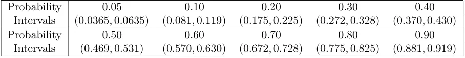
[image:9.595.71.525.344.401.2]Table 1 shows the 95% confidence intervals for different levels of probabilities calculated using the Monte Carlo simulations error based on 1000 simulations. They will help us compare the powers of the different testing procedures as a guide of how large is the simulations error at different levels of power.
Table 1: 95% confidence intervals for different levels of probability.
Probability 0.05 0.10 0.20 0.30 0.40
Intervals (0.0365,0.0635) (0.081,0.119) (0.175,0.225) (0.272,0.328) (0.370,0.430)
Probability 0.50 0.60 0.70 0.80 0.90
Intervals (0.469,0.531) (0.570,0.630) (0.672,0.728) (0.775,0.825) (0.881,0.919)
3.3 Results
3.3.1 Type I error with equal sample sizes
The sample sizes were set equal for both samples and equal to 15, 30, 50 and 100. When the sample sizes were equal to 15 the true Type I error was not achieved by any procedure. Bootstrap calibration however corrected the size of all testing procedures and for the sample sizes. For the sample sizes 30 and 50 we can see that empirical and exponential empirical likelihood calibrated with the F distribution performed better than the other testing procedures. What is more, is that James test when calibrated using an F rather than a corrected χ2 distribution, shows
no significant improvement. Finally, when the sample sizes are large all procedures attain the nominal Type I error of the test.
3.3.2 Type I error with unequal sample sizes
The second sample, which came from the mixture of two Dirichlets, had observations which were less spread (its covariance determinant was smaller) and for this reason it will now have a larger size.
Table 2: Estimated probability of Type I error using different tests and a variety of calibrations. The nominal level of the Type I error was equal to 0.05. The numbers in bold indicate that the estimated probability was within the acceptable limits.
Scenario 1 Scenario 2
Testing Sample sizes Sample sizes
procedure n= 15 n= 30 n= 50 n= 100 n= 15 n= 30 n= 50 n= 100 Hotelling 0.097 0.067 0.073 0.05 0.09 0.083 0.078 0.061 James(χ2) 0.092 0.065 0.069 0.049 0.087 0.08 0.072 0.059 James(F) 0.09 0.065 0.069 0.048 0.078 0.078 0.072 0.059 EEL(χ2) 0.139 0.075 0.075 0.055 0.184 0.112 0.089 0.065 EL(χ2) 0.126 0.066 0.071 0.051 0.154 0.097 0.08 0.062 EEL(F) 0.095 0.056 0.06 0.05 0.114 0.083 0.076 0.062 EL(F) 0.08 0.052 0.054 0.046 0.099 0.072 0.064 0.056 Hotelling(bootstrap) 0.046 0.052 0.061 0.041 0.047 0.055 0.056 0.05
James(bootstrap) 0.044 0.052 0.061 0.041 0.046 0.055 0.056 0.05 EEL(bootstrap) 0.051 0.046 0.058 0.043 0.05 0.059 0.056 0.057
EL(bootstrap) 0.049 0.046 0.057 0.043 0.046 0.054 0.054 0.057
[image:10.595.94.506.465.662.2]is again necessary for the medium sizes. The conclusion is again that the bootstrap computation of the p-values does a very good job.
Table 3: Estimated probability of Type I error using different tests and a variety of calibrations. The nominal level of the Type I error was equal to 0.05. The numbers in bold indicate that the estimated probability was within the acceptable limits.
Scenario 1 Scenario 2
Testing n1 = 15 n1 = 30 n1= 50 n1= 15 n1= 30 n1 = 50
procedure n2 = 30 n2 = 50 n2= 100 n2= 30 n2= 50 n2= 100
Hotelling 0.222 0.154 0.160 0.236 0.189 0.178
James(χ2) 0.142 0.086 0.053 0.106 0.087 0.054
James(F) 0.134 0.08 0.053 0.113 0.089 0.054
EEL(χ2) 0.174 0.08 0.049 0.211 0.128 0.072
EL(χ2) 0.165 0.072 0.043 0.183 0.108 0.065
EEL(F) 0.115 0.053 0.039 0.139 0.089 0.056
EL(F) 0.104 0.045 0.038 0.114 0.076 0.047
Hotelling(bootstrap) 0.078 0.055 0.05 0.073 0.060 0.046 James(bootstrap) 0.075 0.052 0.04 0.062 0.055 0.035 EEL(bootstrap) 0.074 0.041 0.037 0.057 0.062 0.043 EL(bootstrap) 0.072 0.039 0.037 0.052 0.061 0.035
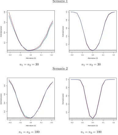
3.3.3 Estimated power of the tests with equal sample sizes
only the bootstrap calibrated procedures. The reason for this is that the testing procedures were size correct when bootstrap calibration was implemented.
In all cases we can see that there little difference between the two quadratic tests when calibrated with bootstrap. What is evident from all testing procedures is that as the sample size increases the powers increase as expected. When looking at the case when the sample size is equal to 30 (Table 4) we see that the power of the quadratic tests is higher than the power of the empirical likelihoods. When the alternative (change in the fourth component) is with a negative sign the power is higher than when the alternative is with a positive sign. But as we move towards the null hypothesis the differences between the two types of testing procedures decrease. When the sample sizes are equal to 100 there are almost no differences between the quadratic tests and the empirical likelihood methods (Table 4).
As seen from Table 3 when the sample sizes are small, no procedure managed to attain the correct size. The F calibration of the empirical likelihoods and bootstrap calibration of all tests decreased the Type I error, yet not enough. When the sample sizes increase, all the empirical likelihood methods estimate the probability of Type I error correctly only when theF
or bootstrap calibration is applied. As for the quadratic tests, bootstrap calibration has proved very useful too. Finally, when the sample sizes are large we can see that Hotelling test is not size correct, as expected (Hotelling assumes equality of the covariance matrices), but all the other testing procedures estimate the probability of Type I error within the acceptable limits regardless of bootstrap calibration.
Table 5 presents the estimated powers of the bootstrap calibrated testing procedures. The empirical likelihood methods with bootstrap was computationally heavy and for this reason we estimated the powers of these two methods only for two sample sizes, 30 and 100.
Similarly to the previous example when both samples have the same size and come from Dirichlet populations the power of the James and Hotelling tests are very similar when boot-strap is employed. When the sample sizes are equal to 30 the quadratic tests exhibit higher powers than than the empirical likelihood methods in the case of a negative change in the first component (see Table 5). This is not true though when the change is positive. In addition, when the negative change gets closer to zero, the power of the empirical likelihood methods is better than the power of the quadratic tests and when the positive change gets closer to zero the opposite is true.
When the sample sizes are large (equal to 100) the quadratic tests and the empirical likeli-hood methods seem to perform equally well as seen in Table 5. But, as the change approaches zero from the negative side, we can see that the tests based on the empirical likelihoods re-ject the null hypothesis more times than the quadratic tests and the converse is true when the change approaches zero from the positive side.
3.3.4 Estimated power of the tests with unequal sample sizes
Table 4: Scenario 1. Estimated powers of the tests with bootstrap calibration when the sample sizes are equal. The alternatives are showed as a function of δ which denotes the change in the 4th component (15).
Sample Testing δ
size procedure -0.21 -0.18 -0.15 -0.12 -0.09 -0.06 -0.03 0.03 0.06 0.09 0.12 0.15 0.18 0.21
n=15 Hotelling(bootstrap) 0.414 0.292 0.194 0.114 0.086 0.050 0.061 0.062 0.082 0.116 0.149 0.206 0.292 0.366 James(bootstrap) 0.410 0.291 0.189 0.114 0.086 0.048 0.061 0.062 0.081 0.115 0.149 0.208 0.291 0.362
Sample Testing δ
size procedure -0.21 -0.18 -0.15 -0.12 -0.09 -0.06 -0.03 0.03 0.06 0.09 0.12 0.15 0.18 0.21
n=30 Hotelling(bootstrap) 0.803 0.606 0.420 0.262 0.153 0.082 0.042 0.069 0.100 0.154 0.258 0.359 0.524 0.630 James(bootstrap) 0.800 0.606 0.420 0.260 0.151 0.082 0.042 0.069 0.101 0.153 0.258 0.356 0.522 0.626 EEL(bootstrap) 0.729 0.555 0.395 0.250 0.145 0.092 0.041 0.061 0.081 0.125 0.229 0.307 0.481 0.583 EL(bootstrap) 0.734 0.554 0.403 0.254 0.144 0.095 0.042 0.063 0.082 0.129 0.234 0.323 0.498 0.600
Sample Testing δ
size procedure -0.21 -0.18 -0.15 -0.12 -0.09 -0.06 -0.03 0.03 0.06 0.09 0.12 0.15 0.18 0.21
n=50 Hotelling(bootstrap) 0.966 0.884 0.726 0.472 0.246 0.111 0.051 0.094 0.117 0.246 0.411 0.582 0.755 0.897 James(bootstrap) 0.966 0.884 0.726 0.472 0.245 0.111 0.051 0.094 0.117 0.245 0.411 0.579 0.755 0.896
Sample Testing δ
size procedure -0.21 -0.18 -0.15 -0.12 -0.09 -0.06 -0.03 0.03 0.06 0.09 0.12 0.15 0.18 0.21
n=100 Hotelling(bootstrap) 1.000 0.995 0.970 0.807 0.527 0.210 0.075 0.099 0.231 0.463 0.755 0.927 0.984 0.999 James(bootstrap) 1.000 0.995 0.970 0.807 0.527 0.210 0.075 0.099 0.231 0.463 0.755 0.927 0.984 0.999 EEL(bootstrap) 1.000 0.995 0.970 0.805 0.527 0.227 0.084 0.093 0.221 0.471 0.768 0.936 0.988 0.999 EL(bootstrap) 1.000 0.995 0.970 0.805 0.530 0.228 0.082 0.094 0.223 0.474 0.771 0.939 0.989 0.999
Table 5: Scenario 2. Estimated powers of the tests with bootstrap calibration when the sample sizes are equal. The alternatives denote the change (δ) in the 1st component (17).
Sample Testing δ
size procedure -0.21 -0.18 -0.15 -0.12 -0.09 -0.06 -0.03 0.03 0.06 0.09 0.12 0.15 0.18 0.21
n=15 Hotelling(bootstrap) 0.546 0.409 0.237 0.152 0.060 0.049 0.037 0.094 0.148 0.244 0.306 0.468 0.593 0.718 James(bootstrap) 0.544 0.408 0.233 0.150 0.060 0.050 0.034 0.091 0.148 0.241 0.304 0.468 0.591 0.716
Sample Testing δ)
size procedure -0.21 -0.18 -0.15 -0.12 -0.09 -0.06 -0.03 0.03 0.06 0.09 0.12 0.15 0.18 0.21
n=30 Hotelling(bootstrap) 0.942 0.833 0.665 0.403 0.214 0.081 0.045 0.103 0.207 0.347 0.530 0.693 0.796 0.889 James(bootstrap) 0.941 0.832 0.663 0.404 0.212 0.081 0.045 0.104 0.207 0.347 0.530 0.694 0.795 0.888 EEL(bootstrap) 0.919 0.817 0.648 0.433 0.251 0.112 0.070 0.100 0.215 0.322 0.511 0.694 0.817 0.884 EL(bootstrap) 0.913 0.813 0.638 0.422 0.236 0.099 0.064 0.102 0.212 0.324 0.519 0.696 0.813 0.886
Sample Testing δ
size procedure -0.21 -0.18 -0.15 -0.12 -0.09 -0.06 -0.03 0.03 0.06 0.09 0.12 0.15 0.18 0.21
n=50 Hotelling(bootstrap) 0.997 0.986 0.919 0.756 0.440 0.200 0.056 0.123 0.276 0.514 0.741 0.901 0.968 0.987 James(bootstrap) 0.997 0.987 0.920 0.755 0.440 0.200 0.057 0.123 0.276 0.515 0.741 0.901 0.968 0.987
Sample Testing δ
size procedure -0.21 -0.18 -0.15 -0.12 -0.09 -0.06 -0.03 0.03 0.06 0.09 0.12 0.15 0.18 0.21
n=100 Hotelling(bootstrap) 1.000 1.000 0.999 0.982 0.817 0.426 0.105 0.169 0.514 0.858 0.988 0.998 1.000 1.000 James(bootstrap) 1.000 1.000 0.999 0.982 0.817 0.426 0.106 0.169 0.514 0.858 0.988 0.998 1.000 1.000 EEL(bootstrap) 1.000 1.000 0.999 0.987 0.835 0.461 0.127 0.146 0.483 0.839 0.986 0.997 1.000 1.000 EL(bootstrap) 1.000 1.000 0.999 0.987 0.837 0.462 0.127 0.143 0.479 0.840 0.986 0.998 1.000 1.000
Scenario 1
−0.2 −0.1 0.0 0.1 0.2
0.2
0.4
0.6
0.8
Alternatives (δ)
Estimated po
w
er
−0.2 −0.1 0.0 0.1 0.2
0.2
0.4
0.6
0.8
1.0
Alternatives (δ)
Estimated po
w
er
n1 =n2 = 30 n1 =n2 = 30
Scenario 2
−0.2 −0.1 0.0 0.1 0.2
0.2
0.4
0.6
0.8
Alternatives (δ)
Estimated po
w
er
−0.2 −0.1 0.0 0.1 0.2
0.2
0.4
0.6
0.8
1.0
Alternatives (δ)
Estimated po
w
er
[image:14.595.101.487.75.518.2]n1 =n2 = 100 n1 =n2 = 100
Figure 1: Estimated powers for a range of alternatives. The sample sizes are equal to (a) 30 and (b) 100 for each sample. The solid horizontal line indicates the nominal level (5%) and the two dashed lines are the lower and upper limits of the simulations error. The black and red lines refer to the Hotelling and James test respectively, the green and blue lines refer to the EEL and EL test respectively.
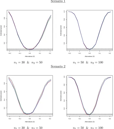
even after bootstrap calibration was applied (see Table 3). Thus, we estimated the powers for the other two combinations of the sample sizes.
Hotelling test seemed to perform slightly better than James in the small samples but in overall there was almost no difference between them. This difference was more obvious in the unequal sample sizes case, where James test showed evidence that is slightly more powerful than Hotelling, especially in the case where the change in the fourth component is positive (see Table 6). When both sample sizes are large though, the powers of the testing procedures are almost the same.
Table 6: Scenario 1. Estimated powers of the tests tests with bootstrap calibration when the sample sizes are different. The alternatives denote the change (δ) in the 4th component (15).
Sample Testing δ
sizes procedure -0.21 -0.18 -0.15 -0.12 -0.09 -0.06 -0.03
n1= 30 Hotelling(bootstrap) 0.958 0.835 0.642 0.400 0.232 0.110 0.052
n2= 50 James(bootstrap) 0.964 0.844 0.644 0.423 0.246 0.115 0.056
EEL(bootstrap) 0.950 0.829 0.627 0.413 0.246 0.122 0.060 EL(bootstrap) 0.951 0.829 0.631 0.418 0.250 0.120 0.063
δ
0.03 0.06 0.09 0.12 0.15 0.18 0.21
n1= 30 Hotelling(bootstrap) 0.058 0.115 0.211 0.336 0.512 0.709 0.831
n2= 50 James(bootstrap) 0.062 0.131 0.225 0.381 0.563 0.754 0.874
EEL(bootstrap) 0.051 0.119 0.216 0.358 0.542 0.731 0.866 EL(bootstrap) 0.050 0.122 0.218 0.367 0.551 0.745 0.873
Sample Testing δ
sizes procedure -0.21 -0.18 -0.15 -0.12 -0.09 -0.06 -0.03
n1= 50 Hotelling(bootstrap) 0.999 0.991 0.934 0.771 0.471 0.196 0.069
n2 = 100 James(bootstrap) 0.999 0.990 0.932 0.766 0.473 0.199 0.074
EEL(bootstrap) 0.998 0.988 0.927 0.762 0.462 0.205 0.082 EL(bootstrap) 0.998 0.989 0.929 0.763 0.466 0.206 0.083
δ
0.03 0.06 0.09 0.12 0.15 0.18 0.21
n1= 50 Hotelling(bootstrap) 0.077 0.176 0.411 0.648 0.852 0.965 0.993
n2 = 100 James(bootstrap) 0.082 0.186 0.440 0.681 0.871 0.974 0.993
EEL(bootstrap) 0.083 0.180 0.434 0.673 0.868 0.971 0.994 EL(bootstrap) 0.088 0.181 0.438 0.677 0.871 0.973 0.995
only James test was size correct after bootstrap calibration (see Table 3). The alternatives in this case were chosen as in the case of equal sample sizes. We chose the second mean of the mixture of two Dirichlet populations and changed it. The second sample (from the mixture of Dirichlet distributions) had always smaller size since its covariance determinant was larger.
When the sample sizes are relatively small, the powers of the quadratic tests is better than the power of the empirical methods regardless of the sign in the change. In fact Hotelling test performs better than James test and it is better when the change in the first component is positive and small. As for the larger sample sizes both quadratic tests and empirical likelihood methods perform very well with. But even then, Hotelling test still performs better than James test when the change in the alternative hypothesis decreases.
4
Discussion and conclusions
Table 7: Scenario 2. Estimated powers of the tests with bootstrap calibration when the sample sizes are unequal. The alternatives denote the change (δ) in the 1st component (17).
Sample Testing δ
sizes procedure -0.21 -0.18 -0.15 -0.12 -0.09 -0.06 -0.03
n1= 50 Hotelling(bootstrap) 0.957 0.868 0.697 0.466 0.245 0.086 0.039
n2= 30 James(bootstrap) 0.940 0.825 0.656 0.417 0.196 0.070 0.040
EEL(bootstrap) 0.924 0.792 0.657 0.437 0.242 0.100 0.060 EL(bootstrap) 0.920 0.790 0.639 0.423 0.225 0.092 0.055
δ
0.03 0.06 0.09 0.12 0.15 0.18 0.21
n1= 50 Hotelling(bootstrap) 0.106 0.245 0.417 0.572 0.752 0.853 0.903
n2= 30 James(bootstrap) 0.092 0.218 0.388 0.534 0.716 0.815 0.866
EEl(bootstrap) 0.095 0.217 0.369 0.514 0.715 0.829 0.883 EL(bootstrap) 0.095 0.220 0.366 0.510 0.717 0.831 0.879
Sample Testing δ
sizes procedure -0.21 -0.18 -0.15 -0.12 -0.09 -0.06 -0.03
n1 = 100 Hotelling(bootstrap) 0.998 0.990 0.940 0.762 0.480 0.222 0.060
n2= 50 James(bootstrap) 0.996 0.982 0.919 0.721 0.441 0.184 0.049
EEL(bootstrap) 0.997 0.988 0.927 0.745 0.482 0.231 0.078 EL(bootstrap) 0.997 0.988 0.925 0.741 0.472 0.223 0.078
δ
0.03 0.06 0.09 0.12 0.15 0.18 0.21
n1 = 100 Hotelling(bootstrap) 0.131 0.307 0.598 0.803 0.943 0.980 0.997
n2= 50 James(bootstrap) 0.112 0.282 0.552 0.758 0.909 0.967 0.986
EEL(bootstrap) 0.103 0.265 0.531 0.753 0.909 0.970 0.988 EL(bootstrap) 0.100 0.259 0.529 0.754 0.907 0.970 0.987
require no numerical optimisation, only matrix calculations and with 299 bootstrap re-samples, the calculation of the p-value requires less than a second. The exponential empirical likelihood requires a few seconds when calibrated using 299 bootstrap samples, whereas the empirical likelihood requires a few minutes.
We proposed the use of the F distribution, with the degrees of freedom of the F distribu-tion as suggested by (Krishnamoorthy and Yu, 2004), for calibradistribu-tion of the empirical and the exponential empirical likelihood test statistics. Our results showed that it works better than the χ2. Another alternative is to use the corrected χ2 distribution (James, 1954). However,
these alternative calibrations do not work when the sample sizes are small or very different. Bootstrap calibration on the other hand, performed very well in almost all cases.
Scenario 1
−0.2 −0.1 0.0 0.1 0.2
0.2
0.4
0.6
0.8
Alternatives (δ)
Estimated po
w
er
−0.2 −0.1 0.0 0.1 0.2
0.2
0.4
0.6
0.8
1.0
Alternatives (δ)
Estimated po
w
er
n1 = 30 & n2 = 50 n1 = 50 & n2= 100
Scenario 2
−0.2 −0.1 0.0 0.1 0.2
0.2
0.4
0.6
0.8
Alternatives (δ)
Estimated po
w
er
−0.2 −0.1 0.0 0.1 0.2
0.2
0.4
0.6
0.8
1.0
Alternatives (δ)
Estimated po
w
er
[image:17.595.101.487.75.512.2]n1 = 30 & n2 = 50 n1 = 50 & n2= 100
Figure 2: Estimated powers for a range of alternatives. The sample sizes are (a) equal ton1= 30
and n2 = 50 and (b) equal to n1 = 50 and n2 = 100. The solid horizontal line indicates the
nominal level (5%) and the two dashed lines are the lower and upper limits of the simulations error. The black and red lines refer to the Hotelling and James test respectively, the green and blue lines refer to the EEL and EL test respectively.
test statistic value. Exponential empirical likelihood on the other hand requires one root search only.
The conclusion that can be drawn is that the Hotelling test statistic or the James test statistic with bootstrap calibration is to be preferred when it comes to algorithmic simplicity and computational cost. Non-parametric likelihood methods perform equally well when bootstrap calibration is present but they require significantly more time than the James or Hotelling test statistics. Furthermore, we can see that the modified (in terms of the calibration) James test performs the same as the classical James test (using a correctedχ2 distribution). Time required
not just personal computers. This could be an evidence against the use of these non-parametric likelihoods.
Based on our simulations we saw that when bootstrap calibration is applied, both methods tend to work almost equally well. If we had high computational power or an algorithm that would perform the empirical and exponential empirical likelihood testing procedures as quick as the James (or the Hotelling) test then we would say that the only reason to choose James test would be because of the convex hull limitation.
The picture we got from the unequal sample sizes is similar to the one in the equal sample size cases. The conclusion drawn from this example is again that empirical likelihood methods are computationally expensive. Bootstrap calibration of the James test requires less than a second when 299 bootstrap re-samples are implemented. Empirical likelihood methods on the other hand require more time which in the case of bootstrap is substantial, especially for the empirical likelihood. Even if we increase the number of bootstrap re-samples, James test will still require maybe a couple of seconds, whereas the empirical likelihood methods will probably require 10 or more minutes.
However, the availability of parallel computing in a desktop computer and a faster imple-mentation of the non parametric likelihood tests, can reduce the time required to bootstrap calibrate the empirical likelihood. Even then, if one takes into account the fact that bootstrap calibration allowed for 299 re-samples it becomes clear that the empirical likelihood is much more computationally expensive. The cost will still be high if data with many observations and or many dimensions are being examined.
References
Aitchison, J. (1982). The statistical analysis of compositional data. Journal of the Royal Statistical Society. Series B, 44(2):139–177.
Aitchison, J. (2003). The statistical analysis of compositional data. Reprinted by The Blackburn Press.
Amaral, G. J. and Wood, A. T. (2010). Empirical likelihood methods for two-dimensional shape analysis. Biometrika, 97(3):757–764.
Baxter, M., Beardah, C., Cool, H., and Jackson, C. (2005). Compositional data analysis of some alkaline glasses. Mathematical geology, 37(2):183–196.
DiCiccio, T. and Romano, J. (1990). Nonparametric confidence limits by resampling meth-ods and least favorable families. International Statistical Review/Revue Internationale de Statistique, 58(1):59–76.
Diciccio, T. J. and Romano, J. P. (1989). On adjustments based on the signed root of the empirical likelihood ratio statistic. Biometrika, 76(3):447–456.
Egozcue, J., Pawlowsky-Glahn, V., Mateu-Figueras, G., and Barcel´o-Vidal, C. (2003). Isometric logratio transformations for compositional data analysis. Mathematical Geology, 35(3):279– 300.
Emerson, S. (2009). Small sample performance and calibration of the Empirical Likelihood method. PhD thesis, Stanford university.
Fisher, N. I., Hall, P., Jing, B.-Y., and Wood, A. T. (1996). Improved pivotal methods for constructing confidence regions with directional data. Journal of the American Statistical Association, 91(435):1062–1070.
Fry, J., Fry, T., and McLaren, K. (2000). Compositional data analysis and zeros in micro data. Applied Economics, 32(8):953–959.
Hall, P. and La Scala, B. (1990). Methodology and algorithms of empirical likelihood. Interna-tional Statistical Review/Revue InternaInterna-tionale de Statistique, 58(2):109–127.
James, G. (1954). Tests of linear hypotheses in univariate and multivariate analysis when the ratios of the population variances are unknown. Biometrika, 41(1/2):19–43.
Jing, B. (1995). Two-sample empirical likelihood method. Statistics & probability letters, 24(4):315–319.
Jing, B. and Robinson, J. (1997). Two-sample nonparametric tilting method.Australian Journal of Statistics, 39(1):25–34.
Krishnamoorthy, K. and Yu, J. (2004). Modified nel and van der merwe test for the multivariate behrens-fisher problem. Statistics & probability letters, 66(2):161–169.
Lancaster, H. (1965). The helmert matrices. American Mathematical Monthly, 72(1):4–12.
Li, X., Chen, J., Wu, Y., and Tu, D. (2011). Constructing nonparametric likelihood confidence regions with high order precisions. Statistica Sinica, 21(4):1767–1783.
Liu, Y., Zou, C., and Zhang, R. (2008). Empirical likelihood for the two-sample mean problem. Statistics & Probability Letters, 78(5):548–556.
Mardia, K., Kent, J., and Bibby, J. (1979). Multivariate Analysis. London: Academic Press.
Owen, A. (1988). Empirical likelihood ratio confidence intervals for a single functional. Biometrika, 75(2):237–249.
Owen, A. (1990). Empirical likelihood ratio confidence regions. The Annals of Statistics, 18(1):90–120.
Owen, A. (2001). Empirical likelihood. Boca Raton: Chapman & Hall/CRC.
Qin, J. and Lawless, J. (1994). Empirical likelihood and general estimating equations. The Annals of Statistics, 22(1):300–325.
Rodrigues, P. C. and Lima, A. T. (2009). Analysis of an european union election using principal component analysis. Statistical Papers, 50(4):895–904.
Scealy, J. L. and Welsh, A. H. (2014). Colours and cocktails: Compositional data analysis 2013 Lancaster lecture. Australian & New Zealand Journal of Statistics, 56(2):145–169.
Tsagris, M. T., Preston, S., and Wood, A. T. A. (2011). A data-based power transformation for compositional data. In Proceedings of the 4rth Compositional Data Analysis Workshop, Girona, Spain.
Zhou, M. (2013). emplik: Empirical likelihood ratio for censored/truncated data. R package version 0.9-9.