Estimation and model selection for left truncated and right censored lifetime data with application to electric power transformers analysis

Munich Personal RePEc Archive

Estimation and model selection for

left-truncated and right-censored lifetime

data with application to electric power

transformers analysis

Emura, Takeshi and Shiu, Shau-Kai

Graduate Institute of Statistics, National Central University, Taiwan

24 July 2014

Estimation and model selection for left-truncated and right-censored

lifetime data with application to electric power transformers analysis

TAKESHI EMURA1, SHAU-KAI SHIU,

Graduate Institute of Statistics, National Central University, Taiwan

In lifetime analysis of electric transformers, the maximum likelihood estimation has been

proposed with the EM algorithm. However, it is not clear whether the EM algorithm offers a better solution compared to the simpler Newton-Raphson algorithm. In this paper, the first

objective is a systematic comparison of the EM algorithm with the Newton-Raphson algorithm in terms of convergence performance. The second objective is to examine the

performance of Akaike's information criterion (AIC) for selecting a suitable distribution among candidate models via simulations. These methods are illustrated through the electric

power transformer dataset.

Keywords

Akaike's information criterion; EM algorithm; lognormal distribution;

Newton-Raphson algorithm; Weibull distribution; Reliability.

Mathematics Subject Classification

62N01, 62N02, 62N05

1. Introduction

Electric power transformers have long lifetime, typically 30 - 40 years under normal operating

conditions, due to their high level of reliability (Zhou 2013). Accordingly, researchers require

long follow-up studies with certain observational constraints, which lead to left-truncation and

right-censoring. Truncation and censoring are common in lifetime data as discussed in the

books by Meeker and Escobar (1998) and Lawless (2003). Recently, Hong, Meeker and

McCalley (2009) carry out lifetime analysis of electric power-transformer data in the US.

Their lifetime data were left-truncated at the starting date of record keeping and

right-censored at the ending date of the study. For this dataset, they propose likelihood

inference and prediction analysis appropriately adjusted for truncation and censoring.

The lognormal and Weibull distributions would be the two most relevant statistical

distributions to model the electric power-transformer data. They have been extensively used

to model lifetime data in the literature. Readers are referred to the books by Crow and

Shimizu (1988) for the lognormal and by Bryan (2006) for the Weibull. They are often fitted

to lifetime data after discriminating between the Weibull and lognormal distributions (e.g.,

Kundu and Manglick 2004; Emura and Wang 2010).

The fitting of the Weibull distribution to the electric power-transformer data is considered

in Hong et al. (2009). They propose a parametric likelihood analysis that properly adjusts for

the sampling bias due to left-truncation and right-censoring. Their study provides a prediction

analysis of the remaining lifetime of the power transformers. Zhou (2013) also considers the

Weibull model for the power transformer data in the absence of truncation.

The fitting of the lognormal distribution to the electric power-transformer data is

developed by Balakrishnan and Mitra (2011). In their paper, the EM algorithm (EM) for

fitting the lognormal distribution to the left-truncated and right-censored data is described.

Under the same model, confidence intervals and prediction intervals are developed using the

show that the EM-based interval has correct coverage rates and is comparable to the intervals

based on the observed information matrix and the parametric bootstrap. The EM is also

developed under the Weibull distribution by Balakrishnan and Mitra (2012). The EM-based

likelihood inference for the gamma and the generalized gamma distribution is developed in

the discussion paper of Balakrishnan and Mitra (2014). The generalized gamma distribution

includes both the Weibull and lognormal distributions as special cases, and hence it provides a

unified framework for performing the EM.

The EM requires mathematical derivation of the expected log-likelihood (E-step) and its

numerical maximization (M-step). In fact, the EM proposed by Balakrishnan and Mitra (2011,

2012) is not simple as it requires some numerical approximations to the M-step. Nevertheless,

the EM often provides stable results when appropriately used. Hence, it is important to clarify

whether the EM offers better solution compared to the simpler Newton-Raphson algorithm.

Checking the adequacy of models is an important issue in parametric analyses. Hong et al.

(2009) used a graphical model checking procedure to verify the Weibull assumption. However,

they did not consider model selection among other candidate distributions. A recently

published Ph.D. thesis of Mitra (2013) and the discussion paper of Balakrishnan and Mitra

(2014) considered model selection via Akaike’s information criterion (AIC) and Bayesian

information criterion (BIC).

The first objective of this paper is to make a comparison between the Newton-Raphson

(NR) method and EM algorithm (EM) under the lognormal and Weibull distributions via

simulations and real data analysis. For the Weibull distribution, we also propose a simplified

NR (called one-dimensional NR), which will be a better alternative to the usual NR and EM.

The second objective of this paper is to investigate Akaike's information criterion (AIC,

Akaike, 1974) to select a suitable model among candidate models. The AIC allows one to

also discussed in the Ph.D. thesis of Mitra (2013) and the discussion paper of Balakrishnan

and Mitra (2014). However, our work is conducted independently and hence supplements

their work under different settings. In fact, the candidate models in our simulations are

different from those in Mitra (2013) and Balakrishnan and Mitra (2014).

The rest of this paper is organized as follows. Section 2 describes the data structure and

the likelihood function. Section 3 introduces the Newton-Raphson and the EM algorithms.

Section 4 defines AIC for model selection. Section 5 presents simulations to compare the NR

and EM algorithms and to examine the performance of AIC. Section 6 analyzes the electric

power transformer datasets. Section 7 concludes the paper.

2. Likelihood construction with left-truncation and right-censoring

In this section, we review the data structures and likelihood construction in the presence of the

left-truncation and right-censoring as considered in Hong et al. (2009) and Balakrishnan and

Mitra (2011, 2012).

2.1 Left-truncated and right-censored data

Data collected on electric power transformers typically involves lower and upper

observational limits, which produces left-truncation and right-censoring respectively. In an

example considered in Hong et al. (2009), the lifetime of the US power transformers are

recorded from 1980 to 2008, a 28 year-period. The interval is still shorter than the average

lifetimes of power transformers of 30 - 40 years under normal operating conditions. Ignoring

censoring and truncation leads to sampling bias.

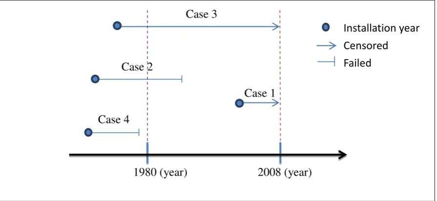
Figure 1 gives an illustration of truncation and censoring. For Case 1, the installation year

of the machine is between 1980 and 2008, and the machine is still in service even after 2008.

Hence, Case 1 is right-censored on 2008. For Case 2, the machine installed before 1980, and

machine is installed before 1980, and it still works after 2008. Hence, Case 3 is both

left-truncated and right-censored. For Case 4, the installation year of the machine and the

failure time of the machine are both before 1980. There is no data available on the lifetime for

Case 4 as the machine is completely missed out of the sampling protocol.

Case 3

Case 2

Case 1

Case 4

[image:6.595.86.534.206.412.2]

1980 (year) 2008 (year)

Figure 1 Example for left truncated and right censored data

2.2 Likelihood construction

To construct the likelihood, we follow the parametric likelihood approaches of Hong et al.

(2009) and Balakrishnan and Mitra (2011, 2012). Note that their likelihoods suitably adjust

for the bias due to left-truncation and right-censoring.

Let X be the original lifetime variable and T log(X) be the log-transformed

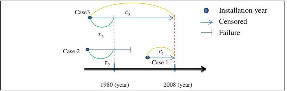
variable. For i-th machine, t_i denotes the observed value for T and c_i denotes the right-

censored time. More precisely, for a machine still in service after 2008, c_i is the time

between the year of installation and the censoring point of 2008 (Figure 2). Let ciL be the

log-transformed right-censored time and _i be the censoring indicator, i.e.,

   

. censored not

is n observatio

the if 1

, censored is

n observatio the

if 0

, ,

δi

Let i be the left-truncated time. More precisely, for a machine installed before 1980, i is

the time between the year of installation and the truncation point of 1980 (Figure 2). Let iL

be the log-transformed left-truncated time and vi be the truncation indicator, i.e.,

   

. truncated not

is n observatio the

if , 1

, truncated is

n observatio the

if , 0

i

v

Further, let S1 and S2 be two index sets, where S1 {i;i 1} is the set of machines

installed after 1980, and S2{i;i 0} is the set of machines installed before 1980.

Case3 c₃

3



Case 2 c₁

₂ Case 1

[image:7.595.79.540.367.514.2]

1980 (year) 2008 (year)

Figure 2 An example for truncated time (i ) and censored time (ci ).

Example 1: Lognormal distribution

We introduce the likelihood under the lognormal distribution. Assume that the

log-transformed lifetime T logX follows a normal distribution with mean  and

standard deviation  0. Then, the likelihood function is

, 1 1 1 1 1 1 ) , ( 1 1 2 1 i i i i L i i S

i _iL

i S i i i y y y y L                                                   _                                  _                                       





where yi min(ti,ciL) and (.) and (.) are the density and distribution function of

the standard normal distribution. The log-likelihood function (without the constant term) is

. 1 log ) 1 ( 1 log ) 1 ( 2 ) ( log 1 log 1 log ) 1 ( 2 ) ( log ) , ( log 1 1 2 2 1 2 2 2









                                                    _                                                       n i n i L i i i i i i n

i iS

L i i i i i v y y y y L                       □

Example 2: Weibull distribution

We introduce the likelihood under the Weibull distribution with the density of X ,

0 , 0 , 0 , exp 1                                _{ }       x x x ,

where  is the scale and  is the shape parameter. The likelihood function is

, exp exp exp exp exp exp ) , ( 1 1 1 1 2 1 i i i i i i S i i i i S i i i i x x x x x x L                                                                                                                                                                                                      





where xi exp( yi ) is the observed lifetime. The log-likelihood function is

Example 3: Exponential distribution

We introduce the likelihood under the exponential distribution, which is a special case of the

Weibull distribution with  1. Therefore, the log-likelihood function is given by

. ) 1 ( log ) ( log 1 1





                  n i i i n i i i v x L       □

In the following, we will use the log-likelihood of each distribution to derive the MLE.

3. Newton-Raphson and EM algorithms

3.1 Newton-Raphson algorithm

If the first-order and second-order derivatives of the log-likelihood are available, one can

maximize the likelihood function using the Newton-Raphson (NR) method. The NR is

suitable to the present problem since all the required derivatives are analytically available.

Example 1: Lognormal distribution

The formulas for the first- and second-order derivatives of the log-likelihood with respect to

the parameters are available in Balakrishnan and Mitra (2011). The MLE of (,  ) is

obtained by sequentially updating the estimate with

                    _   ) , ( ) , ( ) , ( 2 1 1 1 1 k k k k k k f k k k k f f J           ,

where f₁(, )logL(, )/, f₂(, )logL(, )/, and

                             / ) , ( / ) , ( / ) , ( / ) , ( ) , ( 2 2 1 1 f f f f

Jf .

The iteration continues until |k_1k| and |k1k|, for some pre-fixed  0.

We set  0.001 as the stopping criterion for all the simulations.

Example 2: Weibull distribution

The first-order derivatives of the log-likelihood are given by

, ) 1 ( ) , ( log 1 1





                            n i i i n i i i v x L              . log ) 1 ( log log 1 ) , ( log 1 1





                                                             n i i i i n i i i i i v x x x L              

Importantly, the equation logL(, )/ 0 leads to an explicit solution,

. ) )( 1 ( ) ( ˆ 1 1 1 1                    _{ } 







   n i i n i i i n i i v x

Therefore, given k ˆ(k ) , one can obtain a one-dimensional estimating function

0 / ) , ( log )

(  L _k   

f for . We propose a one-dimensional NR to obtain ˆ with

) ( / ) (

1 k k k

k  f  f 

     ,

where f() is defined as



                                                    n i k i k i i k i k i i k v x x L 1 2 2 2 2 2 log ) 1 ( log ) , ( log              .

The iteration stops if |k1k|, for some  0, where we set



0.001 for all the

simulations. The MLE of ˆ is explicitly obtained after finding ˆ. A similar procedure in

the absence of truncation is proposed by Zhou (2013).

Remark II: Although Balakrishnan and Mitra (2012) compare their EM with the NR, their NR

is the usual two dimensional NR using R maxNR routine for their simulations. We rather

Example 3: Exponential distribution

Since the exponential distribution is a special case of the Weibull distribution with  1, we

immediately find the solution to logL()/0 as

. ) )( 1 ( ) 1 ( ˆ ˆ 1 1 1







       _n i i n i i i n i i v x    

There is no need to use the NR. However, the second derivative of the log-likelihood is still

useful to confirm that the solution ˆ is indeed the maximum of the likelihood by

0 / ) ˆ ( log 2

2 _{ }

 L   (Appendix I). □

3.2 EM algorithm

In this section, we briefly introduce the EM algorithm proposed by Balakrishnan and Mitra

(2011, 2012). Let t(t₁,t₂,...,tn ) be the complete log-transformed lifetimes. Since some of

i

t ’s are censored and hence not observed exactly, δ(₁,₂,...,n ) and



(y₁,y₂,...,y_n )

y are observed data. Let θ(, ) be parameters to be estimated.

Example 1: Lognormal distribution

The complete data log-likelihood (without constant terms) is

. 1 log ) 1 ( 2 ) ( log ) , ( log 1 1 2 2





                               n i n i L i i i c v t n L       θ t

The E-step calculates the conditional expectation of the complete data log-likelihood

] , | ) , ( log [ ) ,

(θ θ_k E_θ L_c t θ y δ

Q  _k .

The M-step performs the maximization θk ₁ argmaxQ(θ,θk).

θ  

Balakrishnan and Mitra (2011) suggest a numerical approximation either by a Taylor

until |k1k| and |k1k| for



0.001 as specified for simulations. □

Example 2: Weibull distribution

Let log() and  1/ , where  is the scale parameter and  is the shape

parameter as before. The complete data log-likelihood (without constant terms) is





  

 



 

 

   

 

   

   

   

   



 n

i

n

i

L i i

i i

c v

t t

n L

1 1

exp ) 1 ( exp

log )

, ( log

   

 

 

θ

t .

The formula of the conditional expectation of the complete data log-likelihood Q(θ,θk ) is

a complicated nonlinear function as given explicitly in Balakrishnan and Mitra (2012). They

suggest a linear approximation based on the EM gradient algorithm. The MLE is obtained by

repeatedly calculating θ_{k 1} argmaxQ(θ,θ_k ).

θ 

 □

4. Model selection

Akaike's information criterion or AIC (Akaike, 1974) is a measure of the relative

goodness-of-fit for a given model penalized by the number of parameters in the model. In

particular, AIC is given by AIC2logLˆ2k , where k is the number of unknown

parameters in the model and Lˆ is the maximized value of the likelihood function for the

fitted model. One selects the model with the minimum AIC value.

Another commonly used method for model selection is the Bayesian information criterion

or BIC (Schwarz, 1978) given by BIC2logLˆklogn, where n is the sample size.

Although, AIC and BIC are both simple to apply, their empirical performances are often

different. A comparison of AIC and BIC is given by Burnham and Anderson (2002). In the

biological and social sciences and medicine, they argue that the AIC-type criteria are

reasonable for the analysis of empirical data. BIC might find use in some physical sciences

for general use in the model selection. It is well known that AIC is minimax-rate optimal for

estimating the regression function, and BIC is consistent in selecting the true model (Yang,

2005). In other words, AIC selects the best fitted model and BIC selects the true model.

For a given data, we do not know the true model and even do not know whether the true

model belongs to our candidate models or not. Therefore, we suggest AIC as a general way

for model selection in order to find the best fitted model.

5. Simulations

5.1 Simulation design

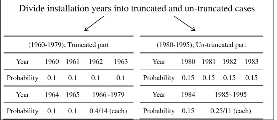
We adopt the simulation design of Balakrishnan and Mitra (2011). We generate the

installation years under the fixed percentage of truncation at 30 or 60%.The set of installation

years are split into two parts: (1960-1979) and (1980-1995). Then, the installation years were

simulated according to the sampling probabilities on Figure 3. For example, suppose that the

sample size is n100, and the percentage of truncation is 30%. Since the truncation year is

fixed at 1980 as in Hong et al. (2009), we generate the installation years that follow the

probability of each year from the truncated part of (1960-1979) with 30 sample sizes, and the

from un-truncated part of (1980-1995) with other 70 sample sizes (Figure 3).

Divide installation years into truncated and un-truncated cases

(1960-1979); Truncated part

Year 1960 1961 1962 1963

Probability 0.1 0.1 0.1 0.1

Year 1964 1965 1966~1979

Probability 0.1 0.1 0.4/14 (each)

(1980-1995); Un-truncated part

Year 1980 1981 1982 1983

Probability 0.15 0.15 0.15 0.15

Year 1984 1985~1995

[image:13.595.79.547.535.738.2]

Probability 0.15 0.25/11 (each)

Then the lifetimes of the machines, in years, are simulated from lognormal, Weibull or

exponential distributions. Adding these lifetimes to the corresponding installation years, we

obtains the failure years of the machines. If the failure year of a machine exceeds 2008, the

machine is censored, where 2008 is the fixed censoring point.

There are some remarks to notice. For the left-truncated machines, if the year of failure is

before 1980, one cannot detect the machine (Case 4 in Figure 1). Therefore, if the year of the

failure is before 1980, we ignore this machine, and generate a new one with the new

installation year and lifetime. The sample sizes used in our simulations are n50, 100, and

200. All the simulation results are based on 1000 Monte Carlo runs. We set the stopping

criterion



0.001 for all the simulations for both NR (Newton-Raphson) and EM (EM

algorithms).

5.2 Results under the lognormal distribution

The lifetimes of the machines are simulated from the lognormal distribution with (, )

being (3.5, 0.5) or (3.0, 0.2), the same values as Balakrishnan and Mitra (2011). We compare

the three algorithms, namely EM1, EM2, NR, where EM1 corresponds to EM algorithm

approximating the hazard function by a Taylor expansion, EM2 corresponds to the EM

gradient algorithm, and NR corresponds to the Newton-Raphson method. The sample mean

and sample standard deviation of yi’s are used as initial values for  and  , respectively.

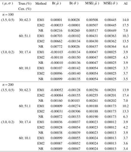
Table 1 compares the results of the three different methods. Overall, the three methods

produce almost unbiased results and have small MSE. As the sample size increases, the bias

and the MSE tend to decrease. This implies that the MLE obtained by the three methods all

work well and the three methods are quite comparable in terms of the bias and MSE. However,

the average number of iterations in the NR is smaller than both EM1 and EM2. This quick

convergence may be regarded as the advantage of the NR over EM1 and EM2.

especially for the NR under small sample sizes and high censoring percentages. In the

following we pick up such a case.

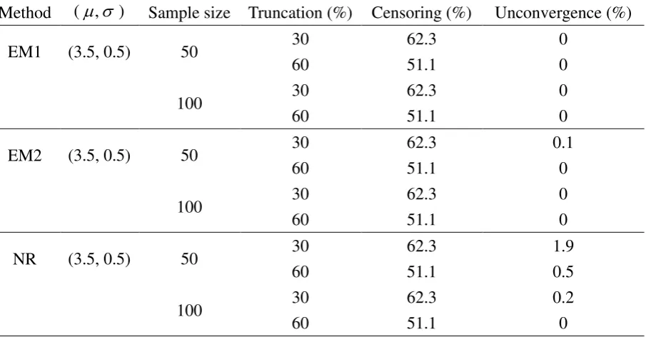
Table 2 gives the separate simulation results under small sample sizes and high censoring

percentage. It can be seen that the NR sometimes produces un-convergence. In spite of the

problem in the NR, the EM1 always converges. Although the percentages of un-convergent

runs in the NR are quite small, the problem may still occur as many engineering applications

have small sample sizes with high censoring percentages.

Table 3 shows the results for the EM1 with n50, where the NR and EM2 occasionally

fail to converge. We see that the EM1 always converges and has reasonable performance for

the bias and MSE. Therefore, under this configuration, only the EM1 works properly.

From Tables 1-3, it can be concluded that, for moderate samples, the EM1, EM2, and NR

perform very similarly in terms of the bias and MSE. However, the NR method converges

more quickly than the EM1 and EM2. Nevertheless, under small sample sizes and high

percentage of censoring, EM1 is the only one reliable method.

[ Insert Tables 1-3 ]

5.3 Results under the Weibull distribution

The lifetimes of the machines are simulated from the Weibull distribution with (, ) being

(35, 3) and (40, 3), which corresponds to (, ) = (3.55, 0.33) and (3.69, 0.33),

respectively. For the Weibull distribution, we denoted T as the log-transformed lifetime

variable which follows an extreme value distribution with parameters  and  . Then

   )

E(T and Var(T)22/6 , where  0.5772 (approximately) is Euler’s

constant. Accordingly, we choose the initial values (0,0) such that

0 0 1

/  





n y

n

i

i and ( ) /( 1) /6

2 0 2 1

2   







n

i

i y n

y .

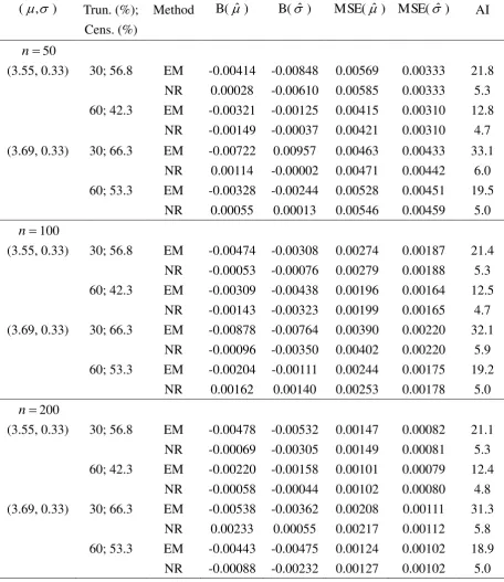
average number of iterations until convergence. It can be observed that the bias and MSE are

very close to zero for both the NR and EM. Hence the accuracy of the EM and NR is virtually

the same. Also, as the sample size increases, the MSE decreases for both methods. A

remarkable difference is that the NR takes fewer steps until convergence than the EM. Unlike

the lognormal distribution, the one-dimensional NR always converges under the Weibull

distribution even for the small sample sizes (n = 50) and high censoring percentage (66.3%).

[ Insert Tables 4 ]

5.4 Model selection performance

We examine the model selection performance of AIC. For instance, if the data is simulated

from lognormal distribution, the MLEs of the three models (lognormal, Weibull and

exponential) are calculated, and then AICs are computed under the three models. Finally, we

select the model that has the smallest AIC among the three. In this case, one may expect that

AIC is the smallest with the lognormal distribution.

Table 5 gives the model selection performance of AIC when the data is simulated from the

lognormal distribution. As expected, the percentage that the lognormal is selected is higher

than the other two. The result is consistent with the observation that the average AIC

calculated under the lognormal distribution is the smallest among the three distributions.

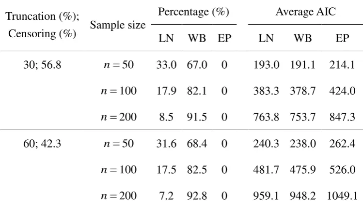
Table 6 shows the performance of AIC when the data is generated from the Weibull

distribution. Again, the percentage of selecting the Weibull model is the highest and the

average AIC calculated under the Weibull model is the smallest among the three distributions.

It should be noted that the mean lifetimes of the data simulated form the lognormal and

Weibull distributions are both near 30. Therefore, we choose the mean parameter  of the

exponential distribution as 30. Table 7 shows the performance of AIC when the data is

simulated from the exponential distribution. As expected, the percentage of selecting the

distribution among the three distributions.

From Tables 5-7, we find that AIC can appropriately identify the correct model and the

percentage of choosing the correct model increases as the sample size increases. Therefore,

the model selection via AIC seems to have a model selection consistency.

[ Insert Tables 5-7 ]

6. Data analysis

The power transformer lifetime data consist of 710 observations with 62 failures from

manufactures (Hong, et al. 2009). Although the original data is not available, their paper

provides a systematic subset of the data containing 286 observations with 39 failures, which is

described in Appendix II.

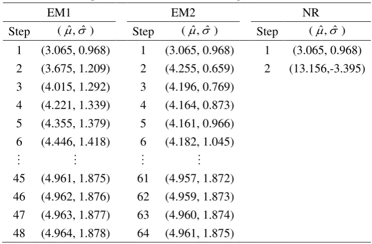
Table 8 shows the successive steps of iterations of the NR and EM (EM1 and EM2) for

fitting the lognormal distribution. We find that the NR diverges at the 2 iteration step. The nd

high censoring percentage (86.4%) explains this phenomenon as the NR occasionally diverges

under small sample sizes and high censoring percentage in the simulations (Section 5). On the

other hand, the two EM algorithms converge and their estimates are very close to one another.

The EM1 converges more quickly than the EM2 does. In all cases, the initial values for the

parameters  and  are taken as the sample mean and sample standard deviation of y_i’s .

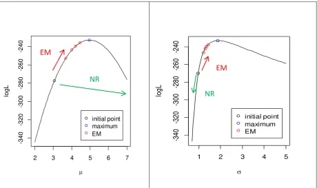
Now, we reveal the detailed behavior of convergence using the EM and NR from Figure 4.

Obviously, the NR moves a wrong way while EM gradually moves to the maximum of the

likelihood. This may be because NR tends to have a big leap in one iteration step. While the

big leap accelerates the convergence speed, it can increase the chance of divergence.

Based on the dataset, we estimate the parameters of the lognormal, Weibull, and

exponential distributions and then compute AIC for the respective models. The resultant AIC

values are 470.04 (lognormal), 472.29 (Weibull) and 470.67 (Exponential). Therefore, we

[image:18.595.83.544.150.423.2]

[ Insert Table 8 ]

Figure 4 The directions of convergence using EM algorithm and NR (Newton-Raphson)

method. The EM algorithm converges to the maximum while the NR algorithm diverges.

7. Conclusion and discussion

The first objective of this paper is to compare the performance of the EM algorithm and

Newton-Raphson method based on the left-truncated and right-censored data. We summarize

the highlights of our finding as follows:

 For the lognormal distribution, when the sample sizes are small and censoring percentage

is high, the Newton-Raphson occasionally fails to converge. On the other hand, the EM

algorithm with the approximation by a Taylor expansion still converges.

 The Newton-Raphson converges more quickly than the EM when both converge.

 The transformer lifetime data analysis demonstrates the real case where the EM

algorithm converges but the Newton-Raphson diverges.

2 3 4 5 6 7

-3

4

0

-3

2

0

-3

0

0

-2

8

0

-2

6

0

-2

4

0

lo

g

L

initial point maximum EM

1 2 3 4 5

-3

40

-3

20

-3

00

-2

80

-2

60

-2

40

lo

gL

initial point maximum EM

EM

NR

EM

 For the Weibull distribution, the proposed one-dimensional Newton-Raphson provides

faster convergence speed than the EM algorithms in any circumstance and the two

algorithms converge to the virtually same limit. Therefore, the EM algorithm appears to

have little advantage over the one-dimensional Newton-Raphson under the Weibull.

Although our comparison between the NR and EM algorithms is based on the

left-truncated and right-censored data, our conclusion (EM is better for lognormal; NR is

better for Weibull; NR is faster when it converges) may be generalized to other data structures

that use EM algorithms for censored data. Obviously, there are many papers that utilize the

EM algorithms for handling censored data. For instance, Ng, Chan, and Balakrishnan (2002)

used EM algorithms to determine the maximum likelihood estimates of the lognormal and

Weibull distributions when data are progressively Type II censored. Recently, Fan and Wang

(2011) and Balakrishnan and Pal (2013) develop EM algorithms for the Weibull analysis

under very general competing risks structures. Since the likelihood in their paper seems to be

twice differentiable, the NR method may still apply. However, it is less clear to us whether our

one-dimensional NR method is appropriate or not for such complicated data structure.

The second objective of this paper is to investigate Akaike's information criterion (AIC)

for model selection. In the simulations, we have confirmed that AIC can correctly identify the

true model among the candidate models. In addition, when the sample size gets large, the

percentage of choosing the correct model increases. Therefore, AIC exhibits model selection

consistency. Note that Barakrishnan and Mitra (2014) also consider AIC as well as BIC as a

model selection tool. Our candidate models in the simulations are exponential, Weibull and

lognormal distributions while those in Barakrishnan and Mitra (2014) are Weibull, lognormal,

gamma, and generalized gamma distributions. Hence, our paper provides additional support

for the performance of AIC under different simulation settings.

variable selection and grouping. For example, Hong et al. (2009) consider a regression model

that includes manufacture ID, insulation class, and cooling system as explanatory variables. It

is possible to apply AIC to select optimal sets of explanatory variables, thought the numerical

performance remains to be studied. One can also use AIC for grouping. Hong et al. (2009)

first split the sample into “Old” and “New” groups, where the Old group mostly consists of

truncated samples and the New group mostly consists of un-truncated samples. Then, they fit

a Weibull model with different shape and scale parameters between the two groups. One may

apply AIC to see whether this split results in a better fit. It is interesting to point out that the

different parameters due to truncation can be associated with the concept of “dependent

truncation” [see Emura and Wang (2012) and references therein; Bakoyannis and Touloumi,

2011]. This implies that truncation has some information about the lifetime. It is also

interesting to consider the effect of “dependent censoring” [see Emura and Chen (2014) and

references therein]. How to incorporate the dependent truncation/censoring information in

model selection of power transformer lifetimes is an interesting topic for further investigation.

Acknowledgments

We would like to thank the editor and anonymous reviewer for their helpful comments that

greatly improved the manuscript. This work was financially supported by the National

Science Council of Taiwan (NSC101-2118-M008-002-MY2).

Appendix I: Confirming that ˆ is indeed the MLE

Under the exponential distribution, the solution to the likelihood equation

0 /

) (

log  

 L   is

0 )

1 (

ˆ

1

1 1

1

          

 

 





 









n

i i n

i

i i n

i

i v

x  

. 0 ] ) 1 ( [

ˆ

1

] ) 1 ( [ 2 ] ) 1 ( [

ˆ

1 )

( log

1 3

1 1

3

ˆ

2 2

    



 _{ }

 

   

 

  

  

 









 



n

i

i i i

n

i

i i i

n

i

i i i

v x

v x

v x

L

 

 

 

 _{ }

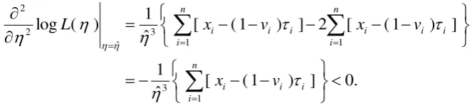
The last inequality holds since xi i (1vi )i for all i.

[image:21.595.145.477.79.155.2]

Appendix II: The subset of data provided by Hong, Meeker, and McCalley (2009)

Table A1 is obtained by reading off numerical values from Fig. 1 of Hong, et al. (2009).

References

Akaike, H. (1974). A new look at the statistical model identification, IEEE Transactions on Automatic Control 19 (6), 716–723.

Bakoyannis G, Touloumi G. (2012). Practical methods for competing risks data: a review. Statistical Method in Medical Research 21, 257-272.

Balakrishnan, N., Mitra, D. (2011). Likelihood inference for lognormal data with left truncation and right censoring with an illustration. Journal of Statistical Planning and Inference 141, 3536-3553.

Balakrishnan, N., Mitra, D. (2012). Left truncated and right censored Weibull data and likelihood inference with an illustration. Computational Statistics & Data analysis 56, 4011-4025.

Balakrishnan, N., Mitra, D. (2013). Some further issues concerning likelihood inference for left truncated and right censored lognormal data. Communications in Statistics-Simulation and Computation 43, 400-416. Balakrishnan, N., Pal, S. (2013). Expectation maximization-based likelihood inference for flexible cure rate

models with Weibull lifetimes. Statistical Methods in Medical Reseach, doi: 10.1177/0962280213491641. Balakrishnan, N., Mitra, D. (2014). EM-based likelihood inference for some lifetime distributions based on left

truncated and right censored data and associated model discrimination. The South African Statistical Journal,

to appear.

Bryan, D. (2006). The Weibull Analysis Handbook, Second Edition, Milwaukee: American Society for Quality, Quality Press.

Burnham, K.P., Anderson, D.R. (2002). Model Selection and Multimodel Inference: A Practical Information-Theoretic Approach, Second ed.

Crow, E.L., Shimizu, K. (1988). Lognormal Distributions: Theory and Applications. Marcel Dekker, New York. Emura, T, Wang, H. (2010). Approximate tolerance limits under the log-location-scale models in the presence of

censoring, Technometrics 52(3), 313-323.

Emura, T. and Wang, W. (2012), Nonparametric maximum likelihood estimation for dependent truncation data based on copulas, Journal of Multivariate Analysis 110, 171-188.

approach, Statistical Methods in Medical Research, doi: 10.1177/0962280214533378.

Fan, T.H., Wang, W.L. (2011). Accelerated Life Tests for Weibull Series Systems With Masked Data. IEEE

Transaction on Reliability 60, No.3.

Hong, Y., Meeker, W.Q., McCalley, J.D. (2009). Prediction of remaining life of power transformers based on left truncated and right censored lifetime data. The Annals of Applied Statistics 3, 857-879.

Kundu, D, Manglick, A. (2004). Discriminating between the Weibull and log-normal distributions, Naval Research Logistics 5, 893-905.

Lawless, J.F. (2003). Statistical Models and Methods for Lifetime Data, Second Edition, New York: John Wiley and Sons.

Mitra, D. (2013). Likelihood inference for left truncated and right censored data. Open Access Dissertations and Theses. Paper 7599.

Meeker, W.Q., Escobar, L.A. (1998). Statistical Methods for Reliability Data. John Wiley & Sons, New York. Ng, H.K.T., Chan, P.S., Balakrishnan, N. (2002). Estimation of parameters from progressively censored data

using EM algorithm. Computational Statistics & Data Analysis 39, 371-386.

Schwarz, G.E. (1978). Estimating the dimension of a model. Annals of Statistics 6 (2), 461–464.

Yang, Y. (2005). Can the strengths of AIC and BIC be shared? A conflict between model indentification and regression estimation, Biometrika 92, 937-950.

[image:23.595.82.523.141.654.2]

Table 1

Bias (B), mean square error (MSE), average number of iterations (AI) for the lognormal distribution using three different methods (EM1, EM2, and NR) in 1000 Monte Carlo

simulations. )

,

(  Trun.(%)

Cen. (%)

Method B(ˆ ) B(ˆ ) MSE(ˆ ) MSE(ˆ ) AI

 n 100

(3.5, 0.5) 30; 62.3 EM1 0.00001 0.00028 0.00508 0.00445 14.0

EM2 -0.00033 -0.00001 0.00507 0.00445 17.5

NR 0.00216 0.00260 0.00517 0.00449 7.0

60; 51.1 EM1 0.00703 -0.00102 0.00431 0.00363 10.3

EM2 0.00662 -0.00134 0.00430 0.00362 13.5

NR 0.00772 0.00026 0.00437 0.00364 6.4

(3.0, 0.2) 30; 17.4 EM1 -0.00103 -0.00134 0.00047 0.00025 3.9

EM2 -0.00110 -0.00150 0.00047 0.00025 4.3

NR -0.00010 -0.00136 0.00047 0.00025 3.9

60; 10.1 EM1 0.00107 -0.00142 0.00054 0.00025 3.7

EM2 0.00096 -0.00140 0.00054 0.00025 3.7

NR 0.00099 -0.00135 0.00054 0.00025 3.5

 n 200

(3.5, 0.5) 30; 62.3 EM1 -0.00052 -0.00128 0.00256 0.00201 13.9

EM2 -0.00084 -0.00155 0.00255 0.00201 17.4

NR 0.00160 0.00103 0.00261 0.00202 7.0

60; 51.1 EM1 0.00009 -0.00274 0.00188 0.00173 10.2

EM2 -0.00031 -0.00306 0.00188 0.00173 13.3

NR 0.00072 -0.00153 0.00190 0.00173 6.3

(3.0, 0.2) 30; 17.4 EM1 0.00036 -0.00037 0.00023 0.00012 3.9

EM2 0.00028 -0.00054 0.00023 0.00012 4.2

NR 0.00038 -0.00039 0.00023 0.00013 3.9

60; 10.1 EM1 0.00099 -0.00055 0.00024 0.00013 3.7

EM2 0.00087 -0.00052 0.00024 0.00013 3.6

NR 0.00089 -0.00047 0.00024 0.00013 3.4

Trun. = Truncation percentage (%); Cens. = Censoring percentage (%);

[image:24.595.87.540.126.362.2]

Table 2

The percentage of unconvergence for the lognormal distribution under three different methods (EM1, EM2, and NR) in 1000 Monte Carlo simulations.

Method (, ) Sample size Truncation (%) Censoring (%) Unconvergence (%)

EM1 (3.5, 0.5) 50 30

60

62.3 51.1

0 0

100 30

60

62.3 51.1

0 0

EM2 (3.5, 0.5) 50 30

60

62.3 51.1

0.1 0

100 30

60

62.3 51.1

0 0

NR (3.5, 0.5) 50 30

60

62.3 51.1

1.9 0.5

100 30

60

62.3 51.1

0.2 0

Unconvergence (%) =100 (the number of un-convergent runs)/1000; 

EM1 = the EM algorithm method approximating the hazard function by the Taylor expansion, EM2 = the EM gradient algorithm,

NR = the Newton-Raphson method.

Table 3

Bias (B), mean square error (MSE), average number of iterations (AI) for the lognormal distribution under the EM1 method for a sample size of 50 in 1000 Monte Carlo simulations.

) ,

(  _Trun.(%);

Cen. (%)

Method B(ˆ ) B(ˆ ) MSE(ˆ ) MSE(ˆ ) AI

 n 50

(3.5, 0.5) 30; 62.3 EM1 0.00235 -0.00594 0.01038 0.00802 14.17

60; 51.1 EM1 0.00372 -0.00712 0.00802 0.00713 10.33

(3.0, 0.2) 30; 17.4 EM1 0.00141 -0.00254 0.00089 0.00050 3.97

60; 10.1 EM1 0.00102 -0.00248 0.00103 0.00052 3.77

[image:24.595.80.523.521.652.2]

[image:25.595.80.537.126.654.2]

Table 4

Bias (B), mean square error (MSE), and average number of iterations (AI) for the Weibull distribution under two different methods (EM and NR) in 1000 Monte Carlo simulations.

) ,

(  Trun. (%);

Cens. (%)

Method B(ˆ ) B(ˆ ) MSE(ˆ ) MSE(ˆ ) AI

 n 50

(3.55, 0.33) 30; 56.8 EM -0.00414 -0.00848 0.00569 0.00333 21.8

NR 0.00028 -0.00610 0.00585 0.00333 5.3

60; 42.3 EM -0.00321 -0.00125 0.00415 0.00310 12.8

NR -0.00149 -0.00037 0.00421 0.00310 4.7

(3.69, 0.33) 30; 66.3 EM -0.00722 0.00957 0.00463 0.00433 33.1

NR 0.00114 -0.00002 0.00471 0.00442 6.0

60; 53.3 EM -0.00328 -0.00244 0.00528 0.00451 19.5

NR 0.00055 0.00013 0.00546 0.00459 5.0

 n 100

(3.55, 0.33) 30; 56.8 EM -0.00474 -0.00308 0.00274 0.00187 21.4

NR -0.00053 -0.00076 0.00279 0.00188 5.3

60; 42.3 EM -0.00309 -0.00438 0.00196 0.00164 12.5

NR -0.00143 -0.00323 0.00199 0.00165 4.7

(3.69, 0.33) 30; 66.3 EM -0.00878 -0.00764 0.00390 0.00220 32.1

NR -0.00096 -0.00350 0.00402 0.00220 5.9

60; 53.3 EM -0.00204 -0.00111 0.00244 0.00175 19.2

NR 0.00162 0.00140 0.00253 0.00178 5.0

 n 200

(3.55, 0.33) 30; 56.8 EM -0.00478 -0.00532 0.00147 0.00082 21.1

NR -0.00069 -0.00305 0.00149 0.00081 5.3

60; 42.3 EM -0.00220 -0.00158 0.00101 0.00079 12.4

NR -0.00058 -0.00044 0.00102 0.00080 4.8

(3.69, 0.33) 30; 66.3 EM -0.00538 -0.00362 0.00208 0.00111 31.3

NR 0.00233 0.00055 0.00217 0.00112 5.8

60; 53.3 EM -0.00443 -0.00475 0.00124 0.00102 18.9

NR -0.00088 -0.00232 0.00127 0.00102 5.0

Trun. = Truncation percentage (%); Cens. = Censoring percentage (%) EM = the EM algorithm

[image:26.595.126.495.155.370.2]

Table 5

The percentage of the model selected by AIC and the average of AIC when the data is

simulated from the lognormal distribution with (, ) = (3.5, 0.5).

Truncation (%);

Censoring (%) Sample size

Percentage (%) Average AIC

LN WB EP LN WB EP

30; 62.3 n50 76.9 20.4 0 172.2 173.8 190.6



n 100 86.0 14.0 0 344.4 347.6 381.4



n 200 91.6 8.4 0 684.9 691.3 759.7

60; 51.1 n50 79.9 20.1 0 216.6 218.2 232.9



n 100 85.6 14.4 0 431.5 434.6 465.3



n 200 92.4 7.6 0 860.8 866.7 928.1

Note: LN = lognormal; WB = Weibull; EP = Exponential; We select the model that has the smallest AIC.

Table 6

The percentage of the model selected by AIC and the average of AIC when data is simulated

from the Weibull distribution with (, ) = (3.55, 0.33).

Truncation (%);

Censoring (%) Sample size

Percentage (%) Average AIC

LN WB EP LN WB EP

30; 56.8 n50 33.0 67.0 0 193.0 191.1 214.1



n 100 17.9 82.1 0 383.3 378.7 424.0



n 200 8.5 91.5 0 763.8 753.7 847.3

60; 42.3 n50 31.6 68.4 0 240.3 238.0 262.4



n 100 17.5 82.5 0 481.7 475.9 526.0



n 200 7.2 92.8 0 959.1 948.2 1049.1

[image:26.595.124.499.490.705.2]

[image:27.595.112.511.126.344.2]

Table 7

The percentage of the model selected by AIC and the average of AIC when the data is

simulated from the exponential distribution with  =30.

Truncation (%);

Censoring (%) Sample size

Percentage (%) Average AIC

LN WB EP LN WB EP

30 ; 43.9 n50 19.0 11.3 69.7 250.8 249.2 248.3



n 100 13.9 12.2 73.9 503.6 499.3 498.3



n 200 8.7 12.8 78.5 989.2 967.3 966.8

60; 41.6 n50 22.0 10.5 67.5 260.0 258.7 257.7



n 100 17.6 11.8 70.6 518.3 515.0 514.0



n 200 9.0 12.2 78.8 1036.4 1028.3 1027.3

Note: LN = lognormal; WB = Weibull; EP = Exponential; We select the model that has the smallest AIC.

Table 8.

The successive steps of iterations of the EM algorithms and Newton-Raphson (NR) method for the lognormal distribution.

EM1 EM2 NR

Step (ˆ,ˆ ) _Step (ˆ,ˆ ) _Step (ˆ,ˆ )

1 (3.065, 0.968) 1 (3.065, 0.968) 1 (3.065, 0.968)

2 (3.675, 1.209) 2 (4.255, 0.659) 2 (13.156,-3.395)

3 (4.015, 1.292) 3 (4.196, 0.769)

4 (4.221, 1.339) 4 (4.164, 0.873)

5 (4.355, 1.379) 5 (4.161, 0.966)

6 (4.446, 1.418) 6 (4.182, 1.045)

   

45 (4.961, 1.875) 61 (4.957, 1.872)

46 (4.962, 1.876) 62 (4.959, 1.873)

47 (4.963, 1.877) 63 (4.960, 1.874)

48 (4.964, 1.878) 64 (4.961, 1.875)

[image:27.595.128.494.458.698.2]

[image:28.595.78.541.129.759.2]

Table A1.

The systematic subset of the transformer lifetime data provided by Hong, Meeker, and McCalley (2009). (Unit: years).

Number of machines Truncation indicator Truncation time

Lifetime Censoring

Number of machines

Truncation indicator

Truncation time

Lifetime Censoring

indicator

Censoring time 22

1 19

5 5 9 3 7 7 8 10

3 2 1 1 1 1

0 0 0 0 0 0 0 0 0 0 0 0 0 0 0 0 0

12 18 16 18 18 20 20 22 24 26 28 30 32 32 38 38 40

41 42 44 46 47 48 49 51 53 55 57 59 60 61 61 66 69

0 1 0 0 0 0 0 0 0 0 0 0 0 0 1 0 0