Dark Matter without Matter

ISSN Online: 2153-120X ISSN Print: 2153-1196

DOI: 10.4236/jmp.2018.913147 Nov. 7, 2018 2320 Journal of Modern Physics

Dark Matter without Matter

Rainer Burghardt

A-2061 Obritz 246, Obritz, Austria

Abstract

We design a cosmological model that expands at a speed less than that of free fall and which allows accelerations of the recession velocity. In addition, the underlying geometry of the model can be adjusted in such a way that attrac-tive forces arise in the cosmos, forces whose sources are not matter. This could explain dark matter as a property of space and one could also address the question of why galactic systems are not subject to expansion.

Keywords

Dark Matter, Cosmology, Accelerated Expansion, Recession Velocity Less Than with Free Falling Expansion

1. Introduction

Careful measurements have proven that there must be attractive forces in the ga-laxies that cannot be explained by the action of mass of the stellar objects. It has been suggested that these forces emanate from matter which does not emit light and therefore one has called the source of these forces as dark matter. Despite 20 years of searching, one has not found matter, and other explanations have not been satisfactory.

We can imagine that the forces do not come from localizable objects, but stem from the geometric structure of space. This concept is in perfect harmony with the principles of general relativity. Gravity, tidal force, and also rotational forces are usually described by the properties of space. In addition, pressure and mass density are derived from geometrical quantities.

Our new approach is based on mathematical methods already hidden in Schwarzschild’s paper on the interior solution (1916). We have worked out these

methods in [1] and [2][3] and have also successfully applied them to the

gravita-tional collapse [4] of the interior Schwarzschild solution. Now we want to apply

the procedure to a cosmological model. We call our model P-model. This model

How to cite this paper: Burghardt, R. (2018) Dark Matter without Matter. Jour-nal of Modern Physics, 9, 2320-2341. https://doi.org/10.4236/jmp.2018.913147

Received: July 13, 2018 Accepted: November 4, 2018 Published: November 7, 2018 Copyright © 2018 by author and Scientific Research Publishing Inc. This work is licensed under the Creative Commons Attribution International License (CC BY 4.0).

http://creativecommons.org/licenses/by/4.0/

DOI: 10.4236/jmp.2018.913147 2321 Journal of Modern Physics

and the Schwarzschild model both are based on the static de Sitter metric as seed metric. In the first case, this metric is a metric on a pseudo-hyper sphere, in the second case it is a metric on a cap of a hypersphere. From both metrics repulsive forces are derivable, which can be interpreted in the dS case as the cause of an expansion. We describe a process that switches these forces from repulsive to at-tractive. Although the elaboration of the P-model requires a considerable amount of mathematics, the underlying physical principles of the Schwarzschild world are well-known, but little respected in the literature.

We note that carrying out this procedure is only possible within the frame-work of the tetrad calculus. Coordinate systems play a minor role, they are only used for basic mathematical operations. In Sec. 2 we briefly outline the static de Sitter model, we explain the use of 4-bein systems, the Ricci-rotation coefficients, and the graded derivative. We discuss the representation of the Einstein field eq-uations in tetrad form and point out that this is useful for many cosmological models and advisable for their clarity. In Sec. 3, we first discuss a static P-model in order to clarify the basic structure of such models. In Sec. 4 and Sec. 5 we de-velop the expanding P-model and discuss it in Sec. 6.

2. Preliminary Remarks

The dS model in its static version is based on a pseudo-hyper sphere with the ra-dius R=const., the polar coordinates

{

}

metric of the dS model in the canonical form is

(

)

2 2 2 2 2 2 2 2 2 2

2 2

2 2 2 2

1

d d d sin d 1 d

1

, 1 1 , 1

R R R R R

s r r r r t

r r

v a v r a

ϑ ϑ ϕ

α

= + + − −

−

= = − = − =

R R

R R

. (2.1)

We identify the quantities vR and αR as the recession velocity of the

galax-ies and the assigned Lorentz factor. From the metric (2.1) we read the 4-bein system

2 3

1 4

1 2 3 4

1 2 3 4

1 2 3 4

, , sin , ,

1 1

, , ,

sin

R R

R R

e e r e r e a

e a e e e

r r

α ϑ

α ϑ

= = = =

= = = = . (2.2)

We use it to calculate the Ricci-rotation coefficients

[ | ] [ | ] [ | ]

t t

s

s j s r j s r j mn j _{n m} nt j _{m r} mt j _{n r}

A =e e +g g e e +g g e e _{, (2.3)}

which we decompose into the radial and the two lateral parts

ˆ

s s s s mn mn mn mn

A =U +B +C _. (2.4)

By means of the unit vectors

{

}

{

}

{

}

{

}

m m m m

m = b = c = u =

(2.5) we continue to decompose into vector quantities

ˆ s ˆ s _{ˆ ,}s s s s_, s s s

mn m n m n mn m n m n mn m n m n

DOI: 10.4236/jmp.2018.913147 2322 Journal of Modern Physics

Finally, we get from (2.3) the geometric quantities

{

}

{

}

(

)

1 _{1,0,0,0 ,} 1 _{sin , cot ,0,0}1

sin

m R m R R R

R R

m m m m

U a v

a

a a

B r C r

r r r r r

α ϑ ϑ ϑ   = = _− _     = = = =     R (2.7)

At the same time, we have executed the operation

i m e_m i

∂ = ∂ _,

with m as a tetrad index and i as a coordinate index (_x4_{=it). The lateral field}

quantities B and C describe the curvatures of the greater circles and the

latitu-dinal circles of the hyper sphere. The quantity Uˆ points away from any point

on the pseudo-hyper sphere. The relations

(

)

|| 2 || 2

|| 2 || 2

1 ˆ ˆ ˆ

1 _, 2

1 _, 3

s s

s s

s s

m n m n mn s s

s s

m n m n mn m n s s

U U U

B B B h B B B

C C C h b b C C C

+ = − + = − + = − + = − + + = − R R R R R (2.8)

are the subequations of Einstein’s field equations. The first relation in (2.8) is the

Friedman equation. hmn=diag

(

)

(

)

mn

g =diag _{. The use of the graded derivatives [4]}

1 2 3

|| | || | || |

ˆ ˆ _, ˆ s _, ˆ s s

n m n m n m n m mn s n m n m mn s mn s

U =U B =B −U B C =C −U C −B C

(2.9) proves to be very advantageous for the representation of field equations. For the Ricci one has

1 2 2

3 3

1 2 3

|| || ||

|| ||

|| || ||

ˆ ˆ ˆ

1 _{ˆ ˆ ˆ}

2

s s s s

mn s s m n n m n m n m s s s s

n m n m n m s s

s s s s s s s s s s s s

R U U U h B B B b b B B B

C C C c c C C C

R U U U B B B C C C

      = −_ + _ −_ + _− _ + _           −_ + _− _ + _           − =_ + _{ }+ + _+_ + _      

. (2.10)

The structures (2.8) and (2.10) can be used for spherically symmetric systems, static, expanding, or collapsing systems. If we reinterpret the cosmological con-stant in the field equations of the dS model, the stress-energy-momentum tensor has the form

2 2 0 3 3 , , mn o p p T p

p κ κµ

µ −    ₋    =_{ } = − = −     R R (2.11)

by using (2.6)-(2.9). p is the pressure and µ0 the matter density of the cosmic

DOI: 10.4236/jmp.2018.913147 2323 Journal of Modern Physics 0 0

p+µ = _.

In one of our papers [5] we have critically examined the dS cosmos concerning

its interpretation. Our P-model is based on the dS model. The above structures are the source for further considerations.

3. The Static P-Model

As a first step towards a generalized model which admits attractive forces, we examine a static cosmological model by introducing the projector technology borrowed from the interior Schwarzschild solution. We do not attribute physical significance to the model. It aims to explain the use of the projectors which we introduce in order to transform repulsive forces into attractive forces. It is the starting point for a more sophisticated model.

We start from the previously described dS model. But now we put

4 4

41 41 1 ˆ1, ˆ1 R R 1

A =U =U =PU U = −α v

R (3.1)

with reference to (2.7). P _{is a space-dependent function which we investigate}

as follows. We call it as a projector.

First, we recalculate the subequations of Einstein’s field equations. For the lat-eral subequations it is sufficient to calculate their timelike components. With

4 0

B = _and C₄=0 _{we get}

2

1 1

4||4 4 4 4|4 44 1 4 4 44 1

1 1 2

1

ˆ R

R R

B B B B U B B B U B

a

U B v

r α

+ = − + = −

 

= = _− _ = −

 R

P

P P

R

and a similar equation for the quantity C. Finally one has

(

)

(

)

2 2

3 3

|| 2 || 2

|| 2 || 2

1 0

0

1 1

0

1 _{, 1} 1

1 _{, 2} 1

s s

m n m n s s

s s

m n m n s s

B B B B B B

C C C C C C

 

 

 

+ = − + = − +

 

 

 

 

 

 

+ = − + = − +

 

 

 

P

P

P

R R

P

R R

. (3.2)

The radial field quantities (3.1) are treated according to

1|1 1 1 1|1 1 |1 1 1

1|1 1 1 1 |1 1 1 1 1

1 |1 1 1

2

ˆ ˆ

ˆ ˆ ˆ ˆ ˆ ˆ ˆ

1 _{ˆ ˆ}

U U U U U U U

U U U U U U U U

U U U

+ = + +

 

= _ + _+ + −

 

= − + _ + − _

P P

P P P P

P P P P

R

.

DOI: 10.4236/jmp.2018.913147 2324 Journal of Modern Physics

(

)

|1= −1 U1

P P _(3.3)

and thus

| 2

1

s s s s

U +U U = −P

R , (3.4)

and finally a relation whose structure is familiar to us from (2.8). We realize that

we get the equations (2.8) of the dS metric for P=1_.

With (3.2) and (3.4) the Ricci tensor

(

)

(

)

(

)

(

)

11 2 2 2

22 2 2 2

33 2

44 2 2 2

2 ₂ 1

1 ₁ 1 ₂ 1

1 2

2 3

R

R

R

R

= + = +

= + + = +

= +

= + =

P

P

R R R

P P

R R R

P R

P P P

R R R

can be calculated and also the Ricci scalar

(

)

(

)

(

)

3 2 3 1 , 1

2

R= +P + P = +P − R= − +P

R R R R

and finally the Einstein tensor

(

)

(

)

(

)

(

)

11 2 2 2

44 2 2 2

1 3 1

2 1 1 2

3 3

3 1

G

G

= + − + = − +

= − + = −

R

P P P

R R R

P _P

R R

.

Therefore the Einstein field equations result in

(

)

1 3

1 2 ,

p

κ = − + P κµ =

R R . (3.5)

For P=1 one again has the pressure and the mass density (2.11) of the dS

model. For later use we note

(

) (

)

2 1 p

κ +µ = −P

R (3.6)

and we finally get the equation of state

(

)

1 1 2 3

p= − + P µ ,

which reduces for P=1 to the equation of state (2.12) of the dS model.

The conservation laws

1 1 1 1 4 4 4 4

|| | 0, || | 0

n n rn n n n rn n n n nr n n n nr n

T =T +A T +A T = T =T +A T +A T =

for this static model are

(

)

|1 0 1, 0 0

p = − p+

µ

µ

DOI: 10.4236/jmp.2018.913147 2325 Journal of Modern Physics

If we differentiate (3.5)

(

)

|1 2 |1 2 1

2 _{2 1}

p U

κ = − P = − −P

R R

we see immediately with (3.7) that (3.8) is satisfied. Thus, the introduction of the

function P has proved to be useful and opens the way to cosmological models

in which the pressure is position-dependent.

4. The Expanding P-Model

In this section we want to show that the static P-model can be extended to an expanding one. We address the problem without reference to conventional cos-mology. We avoid using an expanding metric and the scale factor. Nor do we re-fer to a comoving coordinate system, but we use orthogonal local rere-ference sys-tems. We start from the static de Sitter model. Its metric is the seed metric for our expanding model. In this case, the radius of curvature of the universe will be time-dependent. Then at any moment the expanding cosmos is a snapshot of the dS-cosmos. The coordinate system of the dS-cosmos is completely sufficient to carry out simple mathematical operations. We develop the main part of the theory in the tetrad calculus. This provides reference systems in which the quan-tities of the model have physically interpretable components. We use comoving and non-comoving reference systems. Between them a Lorentz transformation mediates, which includes as a parameter the rate of expansion of the cosmos.

In an earlier paper [5] we have extended the dS model by introducing a second

velocity. We again apply this method, but we abandon the constraint R=const.

which applies to the dS cosmos in order to obtain a genuine expanding model. The double-velocity ansatz is

( )

( )

, , ' , ' ' '

'

R r E r

v = v = R R= T R= R T

R R .

Therein vR =sinη and r=Rsinη is connected to the polar angle η of a

pseudo-hyper sphere. T' is the proper time of an observer who participates in

the expansion of the cosmos. The pseudo-hyper sphere with the time-dependent

radius R forms the skeleton of the cosmological model. r, as in previous

mod-els, is the radial coordinate of the non-comoving observer. vR is, like in the

‘ex-panding’ dS cosmos, the speed of a fictitious freely falling observer. vE and 'R

are to be understood in analogy to the definition of vR, where 'R is another

time-dependent parameter. Thus, we can assume that in a fictive cosmos, which

is preliminary to the physical cosmos, vE has a similar geometric meaning as

R

v has in the dS cosmos. The validity range of the quantities is

' , 0 r

≤ ≤ ∞ ≤ ≤

R R R.

With the ansatz (4.1) we have established the method of double velocities. The

Lorentz transformation

1' 4' 1' 4'

1 , 1 , 4 , 4

L =α L = −i vα L =i vα L =α_{, (4.2)}

DOI: 10.4236/jmp.2018.913147 2326 Journal of Modern Physics

cosmos and the non-comoving observer system m. v is the recession velocity and

α _{the associated Lorentz factor.}

The velocities in (4.1) are supposed to satisfy Einstein’s addition law

, ,

1R E R 1 E E 1R

R E E R

v v v v v v

v v v

v v vv v v

− + −

= = =

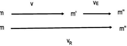
− + − . (4.3)

The composition of the speeds can be taken from the drawing Figure 1.

Figure 1. Composition of the velocities.

The system m’’ is a fictitious reference system in a cosmos that can be

represented by a pseudo-hyper sphere with the radius R. At any given moment,

a snapshot of the cosmos corresponds to the static dS cosmos. This enables us to use the coordinate system of the dS cosmos for basic mathematical operations.

The physical system m’ is the reference system which is in the empirical space

and follows an expansion that is less than that of the free-fall and m the non-comoving reference system. In order to describe all states of motion, we complement (4.2) with

1'' 4'' 1'' 4''

1' 1' 4' 4'

1'' 4'' 1'' 4''

1 1 4 4

, , ,

, , ,

E E E E E E

R R R R R R

L L i v L i v L

L L i v L i v L

α α α α

α α α α

= = − = =

= = − = = . (4.4)

Furthermore, the Lorentz relations

2 2 2

1 1 v , R 1 1 vR, E 1 1 vE

α

α

α

(

)

(

)

(

)

R E v vR E R E vvE E R v vR

α α α= − α =αα + α =α α − _{, (4.6)}

(

)

(

)

(

)

R E R E R R E E E E R R

v v v v v v v v v

α =α α − α =αα + α =α α −

(4.7) apply.

With the definitions in (4.1) one obtains for the recession velocity

2 ' 1

' r r v

r − =

−

R R

R R

. (4.8)

From (4.1) it can be seen that vR accepts the value 1 at the equator of the

pseudo-hyper sphere. That is the speed of light in the natural measuring system.

In [5] we have shown that the velocity can only reach asymptotically the speed of

light, i.e. it can come infinitely close to the value 1 only after an infinitely long

time. Furthermore, we can see from Einstein’s addition law of velocities (4.3) that the recession velocity is lower than the one of free fall

R

DOI: 10.4236/jmp.2018.913147 2327 Journal of Modern Physics

Thus, we have envisaged a cosmological model whose rate of expansion is slower than the ones of the FRW models and whose rate of expansion can be

manipulated with the parameter 'R. Since the recession velocity does not reach

the speed of light and definitely cannot exceed it, there is no violation of the spe-cial theory of relativity and no violation of causality nor is there any galactic island formation.

For the further development of the theory some basic relations are necessary. We are already familiar with

{

}

{

}

{

}

|m 1,0,0,0 R, | 'm ,0,0, R, | ''m R,0,0, R R R

r = a r = α −i v aα r = α −i v aα

(4.9) referring to the geometry of the hyper sphere and the Lorentz transformations (4.2) and (4.4).

In calculating the changes of the two velocities vR and vE, and finally of the

recession velocity v, we must proceed with care. Both quantities contain, apart

from the radial coordinate, the variable quantities R and 'R. Therefore we

define the two quantities

| ' ' " "

| ' ' " "

1 _{, , ,}

1

' ' , ' ' , ' '

'

m m

m m m m m m m m

m m

m m m m m m m m

L L

L L

= = =

= = =

R R R R R R

R

R R R R R R

R

.

With this and with (4.5) and (4.9) we get

{

}

{

}

{

}

{

}

{

}

{

}

| |

| ' ' | ' '

| " " | " "

1,0,0,0 , 1,0,0,0 ' ,

'

,0,0, , ,0,0, ' ,

'

,0,0, , ,0,0, ' .

'

R R

R m R m E m E m

R R

R m R m E m E m

R R

R m R R R R m E m R R R E m

a a

v v v v

a a

v i v v v i v v

a a

v i v v v i v v

α α α α

α α α α

= − = −

= − − = − −

= − − = − −

R R

R R

R R

R R

R R

R R

(4.11) From the above relations, it is obvious that the change of the two speeds has two causes. First, the speeds depend on the position. The recession velocity and thus the redshift of the light of a galaxy is higher, the farther the galaxy is dislo-cated from the observer. Secondly, the recession velocity depends on the

expan-sion of the cosmos, i.e., on the quantities Rm and 'Rm. So we can expect

acce-lerations of expansion, which is suggested by recent observations. We will take a closer look at this problem later.

Now the necessity arises to develop the properties of the quantities (4.10) from

the geometric and the kinematic structure of the model. A look at Figure 1

shows us that for an observer with the velocity vE the system m’ is the rest

frame. Therefore we demand that in analogy to the non-comoving observers of

the dS cosmos [5]

{

}

{

}

{

}

| | '

| "

1 1

,0,0, , 1,0,0,0 ,

' '

1 ,0,0,

'

E m E E m E

E m E E E E

v

v

v i a v a

v i a

α

α

α α

= =

=

R R

R

DOI: 10.4236/jmp.2018.913147 2328 Journal of Modern Physics

applies. Thus, we expect that from the view of the physical observer m’ no

change in time of the velocity vE can be experienced. With this restrictive

con-dition one can calculate 'Rm'. This restriction simplifies the structure of the

model considerably. From (4.12) and (4.11) and using the Lorenz relations we obtain

{

}

{

}

{

}

'

"

' ,0,0, ,

'

' ,0,0, ,

'

' 0,0,0,1 .

'

m R R R

m E E E

m

i i i v

i i i v

i i

α α

α α

 

= − − _ − _

 

 

= − − _ − _

 

 

= − _ − _

 

R

R R

R

R R

R

R R

(4.13)

For the velocity vR, similar constraints would bring us back to the dS cosmos.

In order to determine the quantity Rm from the structure of the model, further

considerations are necessary. First of all, it is evident that the comoving observers

cannot ascertain any position dependency of R. The model is homogeneous

and its curvature is everywhere the same for T'=const._{. So we can put} R_1'=0.

We do not derive our model by solving Einstein’s field equations under specific conditions, but we make assumptions about a particular geometry, we derive from them all necessary quantities. Then we check, whether they satisfy Eins-tein’s field equations. Since a homogeneous world model is based on a spherical space, some of the required quantities are already familiar to us. Thus, we know the expressions for the two lateral field quantities B and C in the system at rest

1

,0,0,0 , , cot ,0,0

R R

m a m a

B C

r r r ϑ

   

=  = 

   .

We do not derive the field quantities of the comoving system from an expand-ing metric, but with a Lorentz transformation from the metric of the static seed system. With

' m' , ' m'

m m m m m m

B =L B C =L C

we obtain the quantities of the comoving system

' R,0,0, R , ' R, cot ,0,1 R

m a a m a a

B i v C i v

r r r r r

α α α ϑ α

   

=_ − _ =_ − _

   . (4.14)

From these relations we realize that the spatial components of these quantities do not appear to be flat. This was the case for the FWR models and the simple

subluminal model, i.e. for all models that expand in free fall. For the special case

0

E

v = _{we get} α α= _R, αR Ra =1 and thus

' 1,0,0, , ' 1 1, cot ,0,

m i m i

B C

r r r ϑ

   

= −  = − 

 R  R.

The spatial parts Bα' and Cα',

(

)

DOI: 10.4236/jmp.2018.913147 2329 Journal of Modern Physics

the free-falling observers.

Let us take another look at the relations (2.4)-(2.7) taking into account (3.1).

To complete the model we need to know the quantity 'U4'. It is decisive for the

development of the universe and enters into the Friedman equation.

The quantity 'U4', which is closely related to the quantity R4', can however

be deduced without further calculation, if we demand that the expansion in all three spatial directions is equal. Thus, after looking at (4.14) one has

4' 4' 4'

'_{U B C i v}aR

r α

∗ ∗

= = = − _{. (4.15)}

For further considerations, we turn to the conservation law. The stress-energy- momentum tensor of the model in the comoving system should have the form of the dS model, if we assume that the matter density has the usual form

2 0 3

κµ = R . For the pressure, we expect a more complicated expression, as the

preliminary study of Sec. 3 shows.

From the conservation law of the moving system with _T4' 'α _=Tα'4'_{=0 and}

4' ' 4' ' 4' ' ' 4' '

|| ' | ' ' ' ' ' ' 0

n n r n n n n n r n

T =T + A T + A T =

follows

(

)

0|4' 3 p 0 'U4' 0

µ + +µ =

(4.16)

using (4.15). On the other hand

0|4' 2 0 4' µ = − µR

follows from the relations 2

0 3

κµ = R . By comparison with (4.16) we get

(

)

0 4' 3₂ p 0 'U4'

µR = +µ

and with (3.6)

(

)

4'= −1 'U4'

R P . (4.17)

Therein P is the projector already used in the last section, which will be

discussed in more detail below. Knowing 'U4' according to (4.15), we have

de-rived the general form of R4' and at the same time we have allowed the model

to expand according to the definition (4.10). Thus,

(

)

4'= −1 −i vα a_rR

 

R P (4.18)

applies.

For P=1 we get back the dS model. Then one has R4'=0 and R=const..

For the two systems m’ and m one finally has

{

}(

)

{

}

(

)

' 0,0,0,1 1 R , ,0,0, 1 R

m = − −i vα a_r  m= −α v −i vα − a_r

 

R P R P .

(4.19) Now we are also able to specify completely the velocity changes. If we substi-tute the above relations into (4.11) we get

{

}

{

}

(

)

{

}

| 1,0,0,0 R ,0,0, 1 R, | ' ,0,0, R

R m a a R m a

v = + α v i vα −P v = α −i vα P

DOI: 10.4236/jmp.2018.913147 2330 Journal of Modern Physics

The 4th _{components of the velocity changes do not vanish. Thus, the P-model}

allows an acceleration of the cosmos.

So far we have developed some quantities necessary for the construction of the theory without much mathematical effort. We now want to put the model on a safe mathematical basis. To this end, we deal in detail with the transformation to the comoving and non-comoving observer systems and with the inhomogeneous transformation law of the Ricci-rotation coefficients. The field quantities are constituents of these Ricci-rotation coefficients, which transform from the

non-comoving system m to the comoving system m’ according to

' ' ' ' ' ' '

' ' ' ' ' ' ' ' ' ' ' ' '| '

' s s ' s, s m n s s, ' s s s m n m n m n m n m n s mn m n s n m

A =A + L A =L A L =L L . (4.21)

The last term in the above relation is called the Lorentz term. This formula

which is fundamental in the tetrad calculus must be generalized to the

P-cosmology so that the Ricci-rotation coefficients Aˆ of the auxiliary model

can be used to generate the Ricci-rotation coefficients A of the P-model. First of

all, we again use the comoving system and now we define most generally the

projector '

'

n m

P . This projector contains only the diagonal components

1' 2' 3' 4'

1' = 2' = 3' =1, 4' =

P P P P P. (4.22)

For the P-cosmology, we modify the inhomogeneous transformation law (4.21) to

' ' ' '

' ' ' ' ' ˆ ' '

' s r r n s s ' s m n m r n s r n m n

A =P L A + L _.

With this we have first accessed the seed metric and we have transformed it into a comoving system. At the same time we have with the help of the projector created a new geometry.

However, it can be seen that this modified transformation law has no effect on

the lateral field quantities B and C. They transform homogeneously and are not

changed by the projector. They are given in the comoving system by (4.14). Thus,

we can concentrate on the quantity U.

If the Ricci-rotation coefficients of the seed model are designated by '

' ' ˆ s

m n

A in

the comoving system, one first obtains

' ' '

' 's r'ˆ' 's

m n m r n

A =P A . (4.24)

Therein

4' 4' 1' 1'

1' 4' ˆ4'1' ˆ1', 4' 1' 1'4'ˆ ˆ4', ˆm' mm' ˆm

U =P A =PU U =P A =U U =L U

is contained. Finally one has

' ,0,0, 1

m R R R R

U = − αα v i v vα α 

 

P

R R . (4.25)

Since the Lorentz transformation is to be interpreted as a pseudo rotation, which takes place in the [1,4]-slice of the surface, the inhomogeneous term can be simplified with hm n' '=diag

{

}

{

}

' ' ' ' 4' 1'

' ' ' ' ' ' ' ' ' 4'1' 1'4'

' s s' ' , 's ' s ' , '

m n m n m n n s n

DOI: 10.4236/jmp.2018.913147 2331 Journal of Modern Physics

From (4.21) only Einstein’s elevator law in cosmology

' ' '

'Um =Um +'Lm

remains.

With a look at (4.2) we calculate with (4.26)

2 2

1' |4' 4' |1'

'L i v=

α

α

and evaluate this with the relation

2_d 2_d 2_d

R R E E

v v v

α =α −α _.

With (4.20), (4.12) we get

2 2 2

1' |4' |4' 4'

2 2

4' |1' |1'

1 '

1 1

'

'

R R E E R R R

R R E E R E

L i v i v v i v

L i v i v i i

α α α α α

α α αα α

= − = −

= − + = − +

R R

R R

.

We define three quantities

{

}

{

}

{

}

' ,0,0, 1, ' 0,0,0,1 _'1 , ' 1,0,0,0 4'

m R m E m R R

G = i vα α αi l = iα f = i vα R

R R , (4.28)

where G describes the change of vR, l the change of vE, and f the change of R.

Finally, one has

' ' ' '

'Lm = −Gm − fm +lm

and with '

' '

m m m m

L = −L L

{

}

{

}

{

}

4'

1 1

0,0,0,1 , ,0,0, , ,0,0,

'

m R m E m R R

G = iα l = −i vα α αi f = α i v i vα α R

R R (4.30)

and the Lorentz term for the inverse transformation

m m m m

L =G + f −l _{. (4.31)}

If we take (4.19) into account we can write

{

}(

)

{

}(

)

' 1,0,0,0 1 1, ,0,0, 1 1.

m R m R

f = −P α αv f = α i vα −P α αv

R R (4.32)

In (4.15) we have deduced that the quantity 'U4' must have the same value as

the quantities B4' and C4' in order to correctly represent the expansion scalar.

Exactly this value would have to be calculated with a Lorentz transformation from the static auxiliary system. We therefore rely on the relation (4.27) and we

calculate the desired quantity using 1 'R=v rE together with

(

)

1

4' 4' 4' 4' 4' 1

4'

1 ˆ

' ' , ,

1 1 1

'

R R

R R R R

U U L U L U i v v

L i i v v i v

r r

α α

αα α α α α

= + = =

= − + − = −

R

R

and indeed we get the expression 'U4'= −i vα a_rR predicted by (4.15).

DOI: 10.4236/jmp.2018.913147 2332 Journal of Modern Physics

(

)

1' 1' 1' 1'

1'

' ' , ,

1 1

' 1

R R

R R R

U U L U v

L v v v

αα

α α α α α α

= + = −

= − − =

P R

P P

R R R

and

(

)

1'

'U =ααR v v− R P= −αE Ev P

R R.

Thus, we have completely calculated the quantity

' 1

'Um = − αE Ev ,0,0,−i vaα R_r

 

P

R . (4.33)

Rather new to FRW models is the radial component in ‘U. Similar to the static

dS cosmos a radial force occurs which can be attractive or repulsive depending

on the sign of P. We realize that with the projector P one can manipulate the

structure of the geometry. We will come back to this later.

After we have succeeded in deriving a complete set of field quantities from the geometry, we want to check whether these quantities satisfy the field equations and the conservation laws and which equation of state results for the cosmos.

It can be seen that we will come across a term P|1' in the progress of the

cal-culations. The analogy to (3.3)

(

)

|1'= −1 'U1'

P P _(4.34)

will prove. After some calculation we find the Friedman equation

1

' '

|| ' ' 2

1

' s ' s '

s s

U +U U = −P

R ,

quite analogous to (3.4). Now the lateral field equations have to be calculated. With the definition of the graded derivatives

1 2

3

' '|| ' '| ' '|| ' '| ' ' ' '

' '

'|| ' '| ' ' ' ' ' ' '

' ' , ' ,

'

s n m n m n m n m m n s

s s n m n m m n s m n s

U U B B U B

C C U C B C

= = −

= − − (4.36)

we get the remaining subequations of Einstein’s field equations

(

)

(

)

2 2

3 3

' '

'|| ' ' ' 2 || ' ' 2

' '

'|| ' ' ' 2 || ' ' 2

1 0

0

1 1

0

1 _{, 1} 1

1 _{, 2} 1

s s

m n m n s s

s s

m n m n s s

B B B B B B

C C C C C C

 

 

 

+ = − + = − +

 

 

 

 

 

 

+ = − + = − +

 

 

 

P

P

P

R R

P

R R

, (4.37)

which, according to the scheme (2.10), we compose to the Ricci tensor and to the Ricci scalar

(

)

DOI: 10.4236/jmp.2018.913147 2333 Journal of Modern Physics

The result is the stress-energy-momentum tensor

' '

0

m n

p p T

p µ −

 

 ₋ 

 

=_{ }

−

 

 

(4.39)

with

(

)

1 3

1 2 ,

p

κ = − + P κµ =

R R . (4.40)

From the conservation law results for the pressure

(

)

|1' 0 ' 1'

p = − p+µ U _{. (4.41)}

From (4.40) we get

(

) (

)

(

)

2 2

1 , '

p p U

κ +µ = −P κ +µ = P

R R .

It follows

(

)

|1'= −1 'U1'

P P ,

thus showing that the ansatz (4.34) is correct. From the conservation law also follows

(

)

0|4' 3 p 0 'U4'

µ = − +µ _{. (4.43)}

With the value (4.40) for µ0 we have previously inferred the relation (4.17).

The relation (3.6) is valid for the expanding model, as well as the equation of state (3.7) of the cosmic fluid

(

)

1 1 2 3

p= − + P µ .

So far, we have worked very successfully with the function P without

speci-fying it. From (4.43) one recognizes that P is closely connected with the

equa-tion of state of the cosmos. By restructuring one gets

0

0 3 1 2

p µ

µ + = −

P . (4.45)

In the literature the relation

0

p w= µ _(4.46)

is common. With this one can write

(

)

(

)

1 _{1 3 ,} 1 _{1 2}

2 w w 3

= − + = − +

P P . (4.47)

It can be seen that the function P _{allows a class of different cosms,}

depend-ing on the choice of the equation of state. We will discuss some specific cases lat-er on.

trans-DOI: 10.4236/jmp.2018.913147 2334 Journal of Modern Physics

formation law

' ' " " ' " ' ' ' ' ' ' " ˆ" " ' ' ' s r r n s" s s

m n m r n s r n m n

A =P L A +l _(4.48)

with

{

}

' ' "

' 's s" s'| ', ' 0,0,0,1 _'

m n s n m m E i

l =L L l = α

R. (4.49)

With this and the Lorentz relations one can easily obtain the already known

quantities of the comoving system m’. However, it must be noted that a return to

the dS auxiliary model is possible only if the conditions for this model are satis-fied, viz R=const., 'R=0.

5. The P-Model in the Non-Comoving System

The cosmologists endeavor to find field quantities and field equations also for the non-comoving system. Although we believe that a representation in the non-comoving system does not provide any new insights, we nevertheless show that such a representation is possible and that the P-model proves to be extreme-ly robust to transformations.

First, the meaning of a non-comoving observer must be clarified. In the lite-rature, one finds the demand r const= ., i.e. the fixing of the radial coordinate r

of the higher-dimensional embedding space. However, it is obvious that such an observer does not comove with the expansion but still moves with respect to an adjacent observer, e.g. to an observer located on the arbitrarily chosen pole of the pseudo-hyper sphere.

For the distance of the non-comoving observer from the pole one has specifically

2 2 0

1 _{d arcsin , sin}

1

r _r

l r r

r

η

η

= = = =

−

∫

R

R .

In an expanding cosmos its radius R depends on time, and its polar angle

η _{also changes if one holds the radial coordinate r tight at a fixed position. Thus,}

the condition r const= . is quite artificial for an expanding cosmos.

In order to complement the P-model in the sense above, field quantities and field equations still have to be revealed in the non-comoving system. The Lorentz transformation is given by (4.2). The lateral field quantities transform homoge-neously and can be taken from (2.7). However, more attention is given to the radial field quantities which transform inhomogeneously according to

'

m m m

U = U +L _.

The L-term

m m m m

L =G + f −l _(5.1)

we have already calculated in (4.30). One now has to perform

' '

' , ' m '

m m m m m m

U = U +L U =L U _{. (5.2)}

One gets

2 2 '

' 1

ˆ _, ˆ _{,0,0,0 ,} m

m m R R m m R R m m m

U = U −α v U = − α v  =L

 

P R R R

DOI: 10.4236/jmp.2018.913147 2335 Journal of Modern Physics

and with this after some calculation the Friedman equation in the non-comoving system

1

|| 2

s s s s

U +U U = − P

R . (5.4)

Comparison with (4.35) shows that the U-equation is form invariant. With

(5.3) we recognize that the radial force U of the non-comoving system does not

reduce to that of the static auxiliary model. That would only be the case if

4'=0

R , i.e., if R=const..

The lateral field equations again are formulated with the graded derivative.

According to (5.3) these equations now contain terms with R|m

(

)

(

)

2

3

2 3

1 1 1 4

|| 2

4 1 1 1

1 1 1 4

|| 2

4 1 1 1

|| 2 || 2

1 0 0 1 1 0 ˆ ˆ 0 1 _, 0 ˆ ˆ ˆ ˆ 0 1 _, 0 ˆ ˆ 1 1

1 , 2 .

m n m n

m n m n

s s s s

s s s s

U U

B B B

U U

U U

C C C

U U

B B B C C C

− −            + = − _{+  }       _{ }   _− + _ − −    _{ }       + = − _{+  }       _{ }   _− + _ + = − + + = − + P P R R R R R R R R R R P P R R (5.5)

From this one gains

(

)

(

)

(

)

11 2 1 1 22 33 2

44 2 1 1 14 1 4

2

1 _ˆ 1

2 2 , 2

3 _{2ˆ , 2 ˆ}

3 2 1

R U R R

R U R U

R

= + + = = +

= − =

= +

P R P

R R R R R P R .

In the non-comoving system, the stress-energy-momentum tensor has the form

(

)

(

)

(

)

2 2

11 0 22 33

2 2 2

41 0 44 0 0

, , ,

, .

T p v p T p T p

T i v p T v p

α

µ

α

µ

µ α

µ

= − − + = − = −

= − + = + + (5.6)

Now all that one has to do is to show how the quite different expressions in (5.5) and (5.6) interrelate. First, we take from (4.45)

0 0 3 1 2 p µ µ +

− =P . (5.7)

Furthermore, we get with (4.19) and (5.3)

(

)(

)

(

)

(

)

(

)

2 2

1 1 0

2

1 1 0

1 1

ˆ

2 2 1

1 1

ˆ

2 2 1

R R R

R R R

U v i v i va v p

r

U v i va i v p

r

α α α α κ µ

α α α α κ µ

DOI: 10.4236/jmp.2018.913147 2336 Journal of Modern Physics

Thus, it can be seen that the stress-energy-momentum tensor (5.6) takes the expected values in the non-comoving system.

6. Discussion of the Model

In the previous section we have set up a cosmological model with the help of a projector, which is formulated very generally. However, there is still the possibil-ity of giving the model a specific appearance by specializing the projector. Now

we assign some specific values to the projector. We recall that P is a function

and a specification can only be made after the model has been worked out.

Case 1:

0 0 0

2 2

3 3

1, w 1, κp , κµ , p µ 0, p µ

= = − = − = + = = −

P

R R .

According to (4.19) one obtains Rm=0, R=const., i.e. a model which is

geometrically represented by a pseudo-hyper sphere of constant radius. In

addi-tion, if is vE =0 one obtains the dS cosmos, i.e. the static model from which

our considerations started.

For a comoving observer in the dS cosmos the polar angle η _{changes on the}

pseudo-hyper sphere. There is a change in position of these observers by a geo-metrically induced drifting.

However, if one has vE ≠0, one obtains the extended dS cosmos, which we

have discussed in detail in [5]. This model is also static, i.e. has constant radius

R _{of the pseudo-hypersphere. However, observer crowds drift apart at a speed}

less than that of free fall.

The motion of the galaxies in this model is accelerated. The Hubble law de-viates from its linear form. This can affect the calculated redshift values. If we take the acceleration into account it may be possible to better adapt the calcu-lated values to the measured ones.

Both models, with or without vE, have the same equation of state. As a result,

no matter flow or energy transport can be detected in the comoving system. Both models have the speed of light as the highest recession velocity, which, however, can only be reached asymptotically. After an infinitely long time, the recession velocity approaches infinitely close the speed of light. The location that can only

be reached by the galaxies asymptotically, i.e. after an infinite time, is the cosmic

horizon. This is the equatorial surface of the hyper sphere, related to the pole of which the observer of the galaxies is located. Any observer can define himself as a pole on the hyper sphere and has his own individual cosmic horizon.

Both models have repulsive forces responsible for the galaxy drift. These forces are directly derived from the dS ansatz.

Case 2:

0 0 0

2 2

1 1 3 1

0, , , , 3 0,

3 3

w κp κµ µ p p µ

= = − = − = + = = −

P

P P .

DOI: 10.4236/jmp.2018.913147 2337 Journal of Modern Physics

forces act in the system in rest of this model, the comoving system is free of forces. The subluminal cosmos expands in free fall; the Einstein elevator

prin-ciple applies [6]. In the non-comoving system the metric has a form from which

can be read the curvature parameter k=1_{. This means that the space is}

posi-tively curved and finite. After a transformation into the comoving system, the

metric has the form k=0_{. This does not mean that the space is flat now. It}

ra-ther means that the free-falling observers do not experience forces, they recog-nize the space to be locally flat, in the same way as the free-falling observers do in the Schwarzschild field.

In this model, the polar angle η _{on the pseudo-hyper sphere does not}

change in time for the comoving observer. With r=_Rsin ,η r=d d 'r T _one

finds

sin cos

r=_R η+_R ηη_.

According to [7] is in this case _R=1 _{and one finally has for the recession}

velocity

sin , 0

v r= = η η= _.

The subluminal model is closely related to the Rh=ct model by Melia.

Me-lia’s calculated redshift values fit the observed values much better than those of FRW models. Therefore, our subluminal model is very close to Nature.

WithvE ≠0 results an extended subluminal model which does not prove to be

particularly useful.

Case 3:

0 0 0

2 2

1 1 3 1

1, , , , 3 0,

3 3

w κp κµ µ p p µ

= − = = = − = =

P

R R .

The pressure in this model is positive. By some authors the equation of state is attributed to an ultra-relativistic gas. What is interesting about this model is that in the comoving system, the system in which we live, an attractive force

1' 1 1' 1'

'E = −αE Ev _R, 'E = −'U

occurs. It corresponds to the repulsive force 'E1'=αE Ev _R1 of the extended dS

model. The corresponding 4th _components

'

'Em of the field quantities are

iden-tical in both models.

This new force depends on the quantity vE. If one puts this quantity zero, this

force vanishes. Then the cosmos expands in free fall. The new attractive force is based on two geometric features of the model: the implementation of a second speed that reduces the recession velocity, and the operation of the projector. The latter changes the sign in (4.33). The attractive force stems from geometry and

may explain the dark matter without our having to assume new types of matter

as the source of this force. Thus, dark matter would be a property of space.

DOI: 10.4236/jmp.2018.913147 2338 Journal of Modern Physics

sphere for the comoving observer. If one recalls the relation r=Rsinη and

R

v =r R one now obtains with cosη=aR=1αR the relations

2

1 _, 1 1

R R

r _r r _{η αv α v}

  = − = −

   



 _R  _R

R R R R R .

The change of the polar angle has two causes: the geometric structure of the model with the forces that occur, and the expansion of the cosmos. With (4.18) the above expression is reduced to

1 v η=_Pα

R.

Depending on the choice of P _{the cases discussed above are included in this}

relation. For P=1 the change of η _{has as the cause the geometric structure}

on the pseudo-hyper sphere and for P=0 _{no temporal change of} η _takes

place.

Let us return to the problem of the recession velocity. Combining (4.11) with (4.19) one has

{

}

{

}(

)

| ' ,0,0, R 0,0,0,1 1 R

R m a a

v = α −i vα + − _i vα _

 

P

R R .

From this it is clear that only for P=0, i.e. for the subluminal model,

|4' 0

R

v = _{results. Since, by definition,} v_E|4' is zero, the recession velocity is also

temporally constant. For other values for P acceleration occurs. It turns out

that both the generalized dS model and the P-model are exact solutions to Eins-tein’s field equations that allow accelerations of the recession velocity.

Further-more, one gets for P= −1 and from _{R=6 1}

(

)

thus also T =0 _{in accordance with the equation of state} µ −₀ 3p=0_.

By recent measurements of the redshift of galaxies one has found that the ex-pansion of the universe is likely to be accelerated. We therefore want to work out how the acceleration for individual models in different frames of reference is ob-tainable. In the textbooks it is mentioned that the acceleration is not covariant,

i.e. it does not transform like vectors between differently moving frames of ref-erence. The problem is rarely discussed in more detail. But we can say that we have already outlined the problem, although it has not been explicitly stated. Ac-celerations are identical to forces on the unit mass. We have already discussed in detail how the forces behave in the various frames of reference. The forces are the field quantities and are components of the Ricci-rotation coefficients. The acce-lerations thus transform according to the inhomogeneous transformation law of the Ricci-rotation coefficients.

With

{

}

{

}

'mn= α,0,0,i vα , 'un= −i vα ,0,0,α

we go into the equations of motion for the comoving observer 'u, represented

in the frame of reference m

( )

|| |4' 4'1' 1' 1' 1'

1

' n' ' s ' '

n s

m u u i αv A L U U

α

DOI: 10.4236/jmp.2018.913147 2339 Journal of Modern Physics

and thus we get the inhomogeneous transformation law of the Ricci-rotation coefficients. In a more conventional way the above relation is written as

1' 1'

1 1 d _'

' d '

D v _{v U U}

DT T

α α

α =α + = .

The total acceleration of a galaxy relative to the non-comoving system is composed of a kinematic component resulting from the motion of the reference systems relative to each other

1' 1 d

'

d '

v L

T α α

=

and a geometric component originating from the basic structure of the model. The latter can be positive, negative, or zero, depending on the value assigned to

the projector. ‘L is the Lorentz term of the inhomogeneous transformation law of

the Ricci-rotation coefficients, which we have got to know in (4.29).

In addition, if one multiplies the last but one equation with the rest mass m0

of the galactic matter, one finally has

0 1' 0 1'

1 1 d _'

' d '

Dmv _{mv m U m U}

DT T

α =α + = .

The kinematic expression contained therein corresponds to the definition of the Lorentz force in the theory of electrodynamics. Finally, one has

' ' Dmv m U

DT =

 _

in referring to classical mechanics. The geometric term and the kinematic term have, according to Sec. 4, the form

1' R R , ' 1' R

U = −αα v P L =α αv P

R R.

The total force 'U U= +'L _{is repulsive for} P=1, i.e. for the extended dS

model, but the kinematic term has the opposite sign and decreases the repulsive

effect. For the simple dS model with v v= R,α α= R, the two terms cancel each

other. The comoving observers are in free fall. For P=0, for the subluminal

model, is 'U =0_{. Thus, no forces act on the comoving observers. For} P= −1

both forces have an attractive effect and add up to

1' 1' E E 1

E = −U = −α v R

and suggest an effect that can be attributed to dark matter.

From the 4th _{component of the equation of motion one obtains with the}

inter-mediate result

|4' i v L' 1'

α = − α

the relation

4

1'

' _'

'

DOI: 10.4236/jmp.2018.913147 2340 Journal of Modern Physics

and after multiplication with the proper mass m0

( )

'

D m m v U DT =

 

one has calculated the work that must be done in transporting the galaxies in the time interval d 'T .

7. Conclusions

A strict geometric treatment of cosmology allows for the ability to modify the underlying geometry to reveal certain physical properties of the cosmos. Thus, the calculated recession velocity of the galaxies can be reduced, enforcing an ac-celeration of these and implementing attractive forces that can be attributed to dark matter. Such forces can also be responsible for ensuring that the internal structures of the galaxies are stable and not subject to the expansion of the un-iverse.

Although the model proposed here is not very close to Nature, it contains ma-thematical methods that prove to be useful in the construction of cosmological models.

Because of the homogeneity of the universe, the new attractive forces are ac-tive throughout the universe and are not limited to galaxies, although this would be desirable. Here one could pursue an idea that was initiated by Einstein and

Strauss [8] and was taken up by some other authors: The insertion of matter

condensates into the homogeneous cosmic fluid.

In additions, the approach with P= −1 seems to be too simple. A look at the

interior Schwarzschild solution, from which we have borrowed the projector

technology, shows that only a more complicated function for P leads to a

func-tioning model. Nevertheless, it is encouraging that three known cosmological

models can be obtained from the P-model, i.e. the dS model, the extended dS

model, and the subluminal model. The P-model leaves open the possibility of de-signing the projector so that the model takes up new structures that may possibly explain the properties of our world.

Conflicts of Interest

The author declares no conflicts of interest regarding the publication of this paper.

References

[1] Burghardt, R. (2006) New Embedding of the Schwarzschild Geometry. II. Interior Solution. Science Edition, Potsdam, 29. http://arg.or.at

[2] Burghardt, R. (2005) Spacetime Curvature. http://members.wavenet.at/arg/EMono.htm

[3] Burghardt, R. (2005) Raumkrümmung. http://members.wavenet.at/arg/Mono.htm [4] Burghardt, R. (1895) Collapsing Schwarzschild Interior Solution. Journal of Modern

Physics, 6, Article ID: 60706. https://doi.org/10.4236/jmp.2015.613195

DOI: 10.4236/jmp.2018.913147 2341 Journal of Modern Physics

Physics, 9, Article ID: 83532. https://doi.org/10.4236/jmp.2018.94047

[6] Burghardt, R. (2016) Einstein’s Elevator in Cosmology. Journal of Modern Physics, 7,Article ID: 72850. https://doi.org/10.4236/jmp.2016.716203

[7] Burghardt, R. (2017) Subluminal Cosmology. Journal of Modern Physics, 8, Article ID: 74922. https://doi.org/10.4236/jmp.2017.84039