doi:10.4236/am.2011.29150 Published Online September 2011 (http://www.SciRP.org/journal/am)
Application of He’s Variational Iteration Method for the
Analytical Solution of Space Fractional Diffusion Equation
Mehdi Safari
Department of Mechanical Engineering, Islamic Azad University, Aligoodarz Branch, Aligoodarz, Iran E-mail: ms_safari2005@yahoo.com
Received July 1, 2011; revised August 3, 2011; accepted August 11, 2011
Abstract
Spatially fractional order diffusion equations are generalizations of classical diffusion equations which are increasingly used in modeling practical super diffusive problems in fluid flow, finance and others areas of application. This paper presents the analytical solutions of the space fractional diffusion equations by varia-tional iteration method (VIM). By using initial conditions, the explicit solutions of the equations have been presented in the closed form. Two examples, the first one is one-dimensional and the second one is two-dimensional fractional diffusion equation, are presented to show the application of the present tech-niques. The present method performs extremely well in terms of efficiency and simplicity.
Keywords:He’s Variational Iteration Method, Fractional Derivative, Fractional Diffusion Equation
1. Introduction
Fractional diffusion equations are used to model prob-lems in Physics [1-3], Finance [4-7], and Hydrology [8-12]. Fractional space derivatives may be used to for-mulate anomalous dispersion models, where a particle plume spreads at a rate that is different than the classical Brownian motion model. When a fractional derivative of order 1 < < 2 replaces the second derivative in a diffusion or dispersion model, it leads to a super diffu-sive flow model. Nowadays, fractional diffusion equa-tion plays important roles in modeling anomalous diffu-sion and subdiffudiffu-sion systems, description of fractional random walk, unification of diffusion and wave propaga-tion phenomenon, see, e.g. the reviews in [1-16], and references therein. Consider a one-dimensional fractional diffusion equation considered in [17]
( , ) ( , )
( ) ( , )
u x t u x t
d x q x t
t x
(1)
on a finite domain xL x xR with 1 2. We
assume that the diffusion coefficient (or diffusivity) . We also assume an initial condition
for
0d x
( , 0
u x t )s x( ) xL x xR
( L,
u x t
and Dirichlet bound-ary conditions of the form and
R . Equation (1)uses a Riemann fractional
derivative of order
)0 ( R, )
u x t b t( )
.
Consider a two-dimensional fractional diffusion
equa-tion considered in [18]
( , , ) ( , , ) ( , )
( , , )
( , ) ( , , )
u x y t u x y t
d x y
t x
u x y t
e x y q x y t
x
(2)
on a finite rectangular domain xL x xH and
L R
y y y , with fractional orders 1 < 2 and
1 < 2, where the diffusion coefficients d x y
, 0
and e x y
, 0
. The “forcing” function q x y
, , t
can be used to represent sources and sinks. We will as-sume that this fractional diffusion equation has a unique and sufficiently smooth solution under the following initial and boundary conditions. Assume the initial con-dition u(x, y, t = 0) = f(x, y) for xL x xH and
L R
y y y , and Dirichlet boundary condition
, ,
, , y t
u x y t B x on the boundary (perimeter) of
the rectangular region xL x xH , L yR
( , , )
L B x y tL
y y
( , , )
B x y t
, with the additional restriction that . In physical applications, this means that the left/lower boundary is set far away enough from an evolving plume that no significant concentrations reach that boundary. The classical dispersion equation in two-dimensions is given by
0
2
. The values of 1 < 2 and
M. SAFARI 1092
the fractional diffusion Equations (1) and (2). The varia-tional iteration method (VIM) established in (1999) by He in [19-22] is thoroughly used by many researchers to handle linear and nonlinear models. The reliability of the method and the reduction in the size of computational domain gave this method a wider applicability. The method has been proved by many authors [23-26], and the references therein, to be reliable and efficient for a wide variety of scientific applications, linear and nonlin-ear as well. The method gives rapidly convergent suc-cessive approximations of the exact solution if such a solution exists. For concrete problems, a few numbers of approximations can be used for numerical purposes with high degree of accuracy. The VIM does not require spe-cific transformations or nonlinear terms as required by some existing techniques. However, we use the VIM to solve fractional diffusion Equations (1) and (2) and fi-nally the results are illustrated in graphical figures.
2. Mathematical Aspects
The mathematical definition of fractional calculus has been the subject of several different approaches [27,28]. The most frequently encountered definition of an integral of fractional order is the Riemann-Liouville integral, in which the fractional order integral is defined as
1 0 d ( ) 1 ( )d ( )
( )
d (
q
t q
t q q
)
f t f
D f t
q
t t
t x
x (3)
while the definition of fractional order derivative is
( )
( ) 0 1
d d ( ) 1 d ( )d
( )
( )
d d d ( )
n n q n
t q
t n n q n n q
f t D f t
n q
t t t t x
f t x
n
(6)
where ( and ) is the order of the opera-tion and n is an integer that satisfies .
q q0 qR
1
n q
3. Basic Idea of He’s Variational Iteration
Method
To clarify the basic ideas of VIM, we consider the fol-lowing differential equation:
LuNug t (5)
where is a linear operator, a nonlinear operator and
L
Ng t an inhomogeneous term. According to VIM, we can write down a correction functional as follows:
1 0 d
t
n n n n
u t u t
Lu Nu g
(6)where is a general Lagrangian multiplier which can be identified optimally via the variational theory. The subscript indicates the n th approximation and is considered as a restricted variation
n un
0
n u
.
4. The Fractional Diffusion Equation Model
and Its Solution by VIM
Now we adopt variational iteration method for solving Equation (1). In the light of this method we assume that
( )
1 0 ( ) ( , ) d
t x
n n n n
u t u t
u d x u q x t (7)where (x) indicates a differential with respect to x
and dot denotes a differential with respect to t, is general Lagrangian multiplier.Similarly, for Equation (2) using variational iteration method, we can obtain
1
( ) ( )
0 ( , ) ( , ) ( , , ) d
n n
t x y
n n n
u t u t
u d x y u e x y u q x y t
(8)5. Numerical Illustrations
5.1. Example 1
Let us consider a one-dimensional fractional diffusion equation for the Equation (1), as taken in [17]
1.8
1.8
( , ) ( , )
( ) ( , )
u x t u x t
d x q x t
t x
(9)
on a finite domain 0 x 1, with the diffusion coeffi-cient
2.8 2.8
( ) (2.2) 6 0.183634
d x x x (10)
the source/sink function
3
( , ) (1 ) t
q x t x e x (11) the initial condition
3
( , 0) ,
u x x for 0 x 1 (12) and the boundary conditions
(0, ) 0, (1, ) t, 0
u t u t e for t (13)
Implementation of Variational Iteration Method for Example 1
Now we consider the application of VIM to one- dimensional fractional diffusion equation with the initial condition of:
3
( , 0) ,
u x x for 0 x 1 (14) Its correction variational functional in x and t can be expressed, respectively, as follows:
(1.8 )
1( , ) ( , ) 0 ( ) ( , ) d
t x
n n n n
u x t u x t
u d x u q x t (15)where (1.8 )x indicates a differential with respect to x
and dot denotes a differential with respect to t, is general Lagrangian multiplier. After some calculations, we obtain the following stationary conditions:
0 (16)
Equation (16) is called Lagrange-Euler equation and Equation (17) is natural boundary condition. The La-grange multiplier can therefore, be identified as 1 and the variational iteration formula is obtained in the form of:
(1.8 )
1( , ) ( , ) 0 ( ) ( , ) d
t x
n n n n
u x t u x t
u d x u q x t (18)We start with the initial approximation of given by Equation (14). Using the above iteration for-mula (18), we can directly obtain the other components as follows:
( , 0)
u x
3 0( , ) ,
u x t x (19)
4 4
1( , ) 1.000001369 ( ),
t
u x t x x te x3x4
(20)
(1.8 )2( , ) 1( , ) 0 1 ( ) 1 ( , ) d
t x
u x t u x t
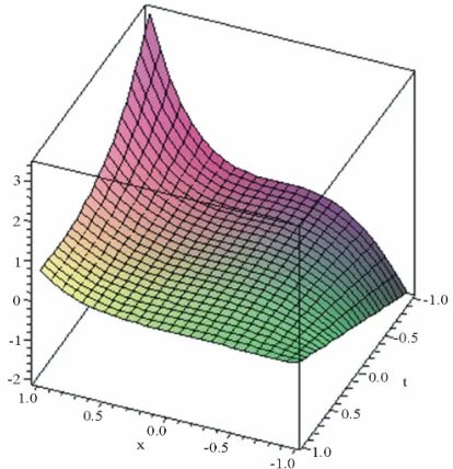
u d x u q x t (21)In Figure 1 we can see the 3-D result of approximate solution of the one-dimensional fractional diffusion equation by VIM.
5.2. Example 2
Let us consider a two-dimensional fractional diffusion equation for the Equation (2), considered in [18].
1.8
1.8
1.6
1.6
( , , ) ( , , ) ( , )
( , , )
+ ( , ) ( , , ),
u x y t u x y t
d x y
t x
u x y t
e x y q x y t
y
(22)
on a finite rectangular domain 0 x 1, , for with the diffusion coefficients
0 y 1
end
[image:3.595.69.276.463.677.2]0 t T
Figure 1. For the one-dimensional fractional diffusion equa- tion with the initial condition (12) of Equation (9), VIM result for u x t( , ).
2.8
( , ) (2.2) / 6
d x y x y (23)
and
2.6
( , ) 2 / (4.6)
e x y x y (24)
and the forcing function
3 3.6
( , , ) (1 2 ) t
q x y t xy e x y (25)
with the initial condition
3 3.6
( , , 0)
u x y x y (26)
and Dirichlet boundary conditions on the rectangle in the
form and
, for all .
3
( , 0, ) (0, , ) 0, ( ,1, ) t ,
u x t u y t u x t e x
3.6
t e y
t0
(1, , )
u y t
Implementation of Variational Iteration Method for Example 2
Again we consider the application of VIM fractional diffusion equation with the initial condition of:
3 3.6
( , 0) ,
u x x y for 0 x 1, 0 y 1 (27)
Its correction variational functional in x and t can be expressed, respectively, as follows:
1
(1.8 ) (1.6 ) 0
( , , ) ( , , )
( , ) ( , ) ( , , ) d
n n
t x y
n n n
u x y t u x y t
u d x y u e x y u q x y t
(28)where (1.8 )x indicates a differential with respect to x, indicates a differential with respect to y and dot denotes a differential with respect to t, also
(1.6 )y
is gen-eral Lagrangian multiplier. After some calculations, we obtain the following stationary conditions:
0 (29)
1 t0 (30)
Equation (29) is called Lagrange-Euler equation and Equation (30) is natural boundary condition. The La-grange multiplier can therefore, be identified as 1
and the variational iteration formula is obtained in the form of:
1
(1.8 ) (1.6 ) 0
( , , ) ( , , )
( , ) ( , ) ( , , ) d
n n
t x y
n n n
u x y t u x y t
u d x y u e x y u q x y t
(31)We start with the initial approximation of given by Equation (27). Using the above iteration for-mula (31), we can directly obtain the other components as follows:
( , 0)
u x
3 3.6 0( , , ) ,
u x y t x y (32)
23 23
4 5 4 5
1
18 23
3 5 4 5
( , , ) 2 2
t 2 t ,
u x y t x y x y t
e x y e x y
M. SAFARI 1094
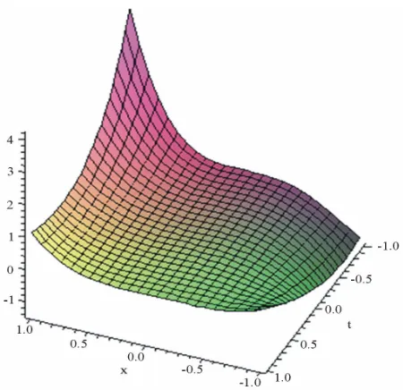
Figure 2. For the two-dimensional fractional diffusion equa-tion with the initial condition (26) of Equation (22), VIM result for u(x t, ) with y1.
2 1
(1.8 ) (1.6 )
1 1 1
0
( , , ) ( , , )
( , ) ( , ) ( , , ) d
t x y
u x y t u x y t
u d x y u e x y u q x y t
(34)In Figure 2 we can see the 3-D result of approximate solution of the one-dimensional fractional diffusion equa-tion by VIM.
6. Conclusions
In this paper, He’s variational iteration method has been successfully applied to find the solution of space frac-tional diffusion equation. All cases show that the results of the VIM method are very good and the obtained solu-tions are shown graphically. In our work, we use the Maple Package to calculate the functions obtained from the He’s variational iteration method.
7. References
[1] R. Metzler, E. Barkai and J. Klafter, “Anomalous Diffu-sion and Relaxation Close to Thermal Equilibrium: A Fractional Fokker-Planck Equation Approach,” Physics Review Letters, Vol. 82, No. 18, 1999, pp. 3563-3567. doi:10.1103/PhysRevLett.82.3563
[2] R. Metzler and J. Klafter, “The Random Walk’s Guide to Anomalous Diffusion: A Fractional Dynamics Approach,” Physics Reports, Vol. 339, No. 1, 2000, pp. 1-77.
doi:10.1016/S0370-1573(00)00070-3
[3] R. Metzler and J. Klafter, “The Restaurant at the End of the Random Walk: Recent Developments in the Descrip-tion of Anomalous Transport by FracDescrip-tional Dynamics,”
Journal of Physics A, Vol. 37, No. 31, 2004, pp. 161-208.
[4] R. Gorenflo, F. Mainardi, E. Scalas and M. Raberto, “Fractional Calculus and Continuous-Time Finance. III. The Diffusion Limit,” Mathematical Finance, Konstanz, 2000, pp. 171-180.
[5] F. Mainardi, M. Raberto, R. Gorenflo and E. Scalas, “Fractional Calculus and Continuous-Time Finance II: The Waiting-Time Distribution,” Physica A, Vol. 287, no. 3-4, 2000, pp. 468-481.
doi:10.1016/S0378-4371(00)00386-1
[6] E. Scalas, R. Gorenflo and F. Mainardi, “Fractional Calcu-lus and Continuous-Time Finance,” Physica A, Vol. 284, No. 1-4, 2000, pp. 376-384.
doi:10.1016/S0378-4371(00)00255-7
[7] M. Raberto, E. Scalas and F. Mainardi, “Waiting-Times and Returns in High Frequency Financial Data: An Em-pirical Study,” Physica A, Vol. 314, No. 1-4, 2002, pp. 749-755. doi:10.1016/S0378-4371(02)01048-8
[8] D. A. Benson, S. Wheatcraft and M. M. Meerschaert, “Application of a Fractional Advection Dispersion Equa-tion,” Water Resource Research, Vol. 36, No. 6, 2000, pp. 1403-1412. doi:10.1029/2000WR900031
[9] B. Baeumer, M. M. Meerschaert, D. A. Benson and S. W. Wheatcraft, “Subordinated Advection-Dispersion Equa-tion for Contaminant Transport,” Water Resource Re-search, Vol. 37, No. 6, 2001, pp. 1543-1550.
[10] D. A. Benson, R. Schumer, M. M. Meerschaert and S. W. Wheatcraft, “Fractional Dispersion, Lévy Motions, and the MADE Tracer Tests,” Transport in Porous Media, Vol. 42, No. 1-2, 2001, pp. 211-240.
doi:10.1023/A:1006733002131
[11] R. Schumer, D. A. Benson, M. M. Meerschaert and S. W. Wheatcraft, “Eulerian Derivation of the Fractional Advec-tion-Dispersion Equation,” Journal of Contaminant Hy-drology, Vol. 48, No. 1-2, 2001, pp. 69-88.
doi:10.1016/S0169-7722(00)00170-4
[12] R. Schumer, D. A. Benson, M. M. Meerschaert and B. Baeumer, “Multiscaling Fractional Advection-Dispersion Equations and Their Solutions,” Water Resource Re-search, Vol. 39, No. 1, 2003, pp. 1022-1032.
[13] A. Carpinteri and F. Mainardi, “Fractals and Fractional Calculus in Continuum Mechanics,” Springer-Verlag, Wien, New York, 1997, pp. 291-348.
[14] F. Mainardi and G. Pagnini, “The Wright Functions as Solutions of the Time Fractional Diffusion Equations,” Applied Mathematics and Computation, Vol. 141, No. 1, 2003, pp. 51-62. doi:10.1016/S0096-3003(02)00320-X [15] O. P. Agrawal, “Solution for a Fractional Diffusion-Wave
Equation Defined in a Bounded Domain,” Nonlinear Dy-namics, Vol. 29, No. 1-4, 2002, pp. 145-155.
doi:10.1023/A:1016539022492
[16] W. R. Schneider and W. Wyss, “Fractional Diffusion and Wave Equations,” Journal of Mathematical Physics, Vol. 30, No. 1, 1989, pp. 134-144. doi:10.1063/1.528578 [17] M. M. Meerschaert, H. Scheffler and C. Tadjeran, “Finite
Vol. 211, No. 1, 2006, pp. 249-261. doi:10.1016/j.jcp.2005.05.017
[18] C. Tadjeran, M. M. Meerschaert and H. Scheffler, “Finite Difference Methods for Two-Dimensional Fractional Dispersion Equation,” Journal of Computational Physics, Vol. 213, No. 1, 2006, pp. 205-213.
doi:10.1016/j.jcp.2005.08.008
[19] J. H. He, “Some Asymptotic Methods for Strongly Nonlinear Equations,” International Journal of Modern Physics B, Vol. 20, No. 10, 2006, pp. 1141-1199.
doi:10.1142/S0217979206033796
[20] J. H. He, “Approximate Analytical Solution for Seepage Flow with Fractional Derivatives in Porous Media,” Computer Methods in Applied Mechanics and Engineer-ing, Vol. 167, No. 1-2, 1998, pp. 57-68.
doi:10.1016/S0045-7825(98)00108-X
[21] J. H. He, “Variational Iteration Method for Autonomous Ordinary Differential Systems,” Applied Mathematics and Computation, Vol. 114, No. 2-3, 2000, pp. 115-123. doi:10.1016/S0096-3003(99)00104-6
[22] J. H. He and X. H. Wu, “Construction of Solitary Solution and Compacton-Like Solution by Variational Iteration Method,” Chaos, Solitons & Fractals, Vol. 29, No. 1, 2006, pp. 108-113.
[23] D. D. Ganji, E. M. M. Sadeghi and M. Safari, “App- lica-tion of He’s Varialica-tional Iteralica-tion Method and Adomian’s
Decomposition Method Method to Prochhammer Chree Equation,” International Journal of Modern Physics B, Vol. 23, No. 3, 2009, pp. 435-446.
doi:10.1142/S0217979209049656
[24] M. Safari, D. D. Ganji and M. Moslemi, “Application of He’s Variational Iteration Method and Adomian’s De-composition Method to the Fractional Kdv-Burgers- Kuramoto Equation,” Computers and Mathematics with Applications, Vol. 58, 2009, pp. 2091-2097.
doi:10.1016/j.camwa.2009.03.043
[25] D. D. Ganji, M. Safari and R. Ghayor, “Application of He’s Variational Iteration Method and Adomian’s De-composition Method to Sawada-Kotera-Ito Seventh-Order Equation,” Numerical Methods for Partial Differential Equations, Vol. 27, No. 4, 2011, pp. 887-897.
doi:10.1002/num.20559
[26] M. Safari, D. D. Ganji and E. M. M. Sadeghi, “Application of He’s Homotopy Perturbation and He’s Variational Iteration Methods for Solution of Benney-Lin Equation,” International Journal of Computer Mathe- matics, Vol. 87, No. 8, 2010, pp. 1872-1884.
doi:10.1080/00207160802524770
[27] I. Podlubny, “Fractional Differential Equations,” Aca-demic Press, San Diego, 1999.