doi:10.4236/jilsa.2011.34022 Published Online November 2011 (http://www.SciRP.org/journal/jilsa)
Parallel Evaluation of a Spatial Traversability Cost
Function on GPU for Efficient Path Planning
Stephen Cossell, Jose Guivant
School of Mechanical and Manufacturing Engineering, The University of New South Wales, Sydney, Australia. Email: {macgyver, j.guivant}@unsw.edu.au
Received March 22nd, 2011; revised September 19th, 2011; accepted October 9th, 2011.
ABSTRACT
A parallel version of the traditional grid based cost-to-go function generation algorithm used in robot path planning is introduced. The process takes advantage of the spatial layout of an occupancy grid by concurrently calculating the next wave front of grid cells usually evaluated sequentially in traditional dynamic programming algorithms. The algorithm offers an order of magnitude increase in run time for highly obstacle dense worst-case environments. Efficient path planning of real world agents can greatly increase their accuracy and responsiveness. The process and theoretical analysis are covered before the results of practical testing are discussed.
Keywords: GPGPU, Dynamic Programming, Concurrent Programming, Path Planning
1. Introduction
Global path planning is an important part of robot navi-gation through both static and dynamic environments. Many simple techniques exist for immediate obstacle avoidance [1], but without a high level path to follow to a desired destination an agent cannot guarantee near opti- mal travel. A current popular technique is to generate a two-dimensional occupancy grid based on the robot’s on- board sensing capabilities, such as laser range scanners [2-4]. On this occupancy grid a cost-to-go function is generated from a single destination point to any number of locations. A global holonomic path can be generated from this function by travelling from grid cell to grid cell by choosing the neighbour with the lowest global cost.
Generation of the cost-to-go function from an occu-pancy grid is an inherently sequential algorithm as the global cost of a cell depends on the calculation of a nei- ghbour closer to the destination point. This paper pre-sents a modified version of the cost-to-go generation al- gorithm that makes use of the parallel hardware found on modern graphics cards, while maintaining numerically identical results to traditional sequential dynamic program- ming algorithms. This paper begins by giving a back-ground on developing concurrent algorithms on modern graphics hardware, followed by a literature review of ex- isting sequential techniques. The paper then demonstrates how the proposed method achieves an order of magnitu- de increase in efficiency before showing experimental
results and their practical benefit.
2. Background
Current forefront central processing unit (CPU) technol- ogy is making use of multiple cores to improve perform- ance and as such many software developers are attempt- ing to find new methods to parallelise existing algorithms for the new paradigm [5,6]. Running along side this CPU evolution in recent years is the growth of graphics hard- ware in capability and performance. This growth has been driven by market forces such as consumer demand for more realistic games and interactive media, but it has enabled a new research area known as General Purpose Computing on Graphics Processing Units (GPGPU) [7]. This section will give a brief outline of some foundation ideas of the field of GPGPU.
2.1. General Purpose Computing on Graphics Processing Units
the same transformation, colouring, texture interpolation and lighting calculations on many different vertices and fragments in a three-dimensional scene. From one point of view, this can be seen as limiting the flexibility of the hardware. On the other hand, it relieves the programmer from having to deal with a core problem associated with concurrent programming.
The two main problems faced by concurrent progra- mmers are concurrent access of critical resources, such as common data, and synchronisation between the indepen- dent threads of execution. Graphics hardware removes the burden of concurrent data access by using the SIMD paradigm and enforces synchronisation at a regular inter- val via the rendering of a single frame to screen or other texture buffer.
Some common programming constructs are known un- der different terminology in a GPGPU context. Memory is usually referred to as either a texture or a frame buffer as the programmer usually accesses data in this memory via pixel or texel lookups.1 A single program run on each
pixel individually is known as a shader program from a traditional graphics programming perspective, or more recently a kernel in GPGPU research.
A common example demonstrating the power of con- current programming on GPU is the grey scaling of an image. For an image that is n × n pixels a sequential al- gorithm will have to process each pixel individually and average the red, green and blue channels to calculate the grey scale intensity. Therefore, the sequential algorithm runs in O(n2) time. On a GPU, since each pixel’s calcula-
tion is independent this kernel can be run on each pixel concurrently, therefore running in O(1) time.2 Analysis
of similar computer vision methods ported to GPU are referred to in [9].
Another textbook example is matrix-matrix multipli-cation [10,11]. Usually a sequential algorithm will run in
O(n3) as each of the n × n cells in the solution matrix
requires a process running in O(n) time (the sum of n
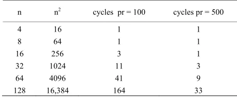
[image:2.595.306.537.112.207.2]multiplications). Again, this kernel can be run on each cell in the solution matrix independently, so a parallel implementation of this process will run in O(n) time. Of course, in practice, this linear algorithm would run slightly slower depending on the number of processors available. For example, many current consumer graphics cards have approximately one hundred thread processors, whereas a high end General Purpose GPU such as the nVidia Tesla [12] has around five hundred thread proc-essors. Table 1 shows the increase in cycles based on the
Table 1. Comparison of cycles required for differing num- ber of available processors.
n n 2 cycles pr = 100 cycles pr = 500
4 8 16 32 64 128
16 64 256 1024 4096 16,384
1 1 3 11 41 164
1 1 1 3 9 33
number of calculations to be completed spread over the number of processors available.
More generally this can be specified as the complexity of the sequential algorithm divided by the number of pro- cessors available. For current consumer graphics hard-ware this means the matrix-matrix multiplication algori- thm could run anywhere between O(n3) and O(n) time
depending on the size of n relative to the number of thr- ead processors. However, with no modification to the al- gorithm itself, this can reach O(n) in current forefront graphics hardware and therefore next generation consu- mer and mobile graphics hardware.
2.2. The Ping-Pong Method
In GPGPU, many simple algorithms require a single iter- ation or frame to be calculated, like image grey scaling or matrix-matrix multiplication. There are however many algorithms that have to be evaluated through a series of steps.3 The state of each step must be saved in a frame
buffer ready for the next calculation. A textbook method outlined in [13] is the ping-pong method. This method uses the standard two texture/buffer approach of having one input buffer and one output buffer, rather than out-putting to screen like normal graphics operations. The difference is that between each step the roles of the two buffers are reversed so that the input from one step be-comes the output of the next step. By have one texture as read-only and the other write-only in each iteration, each kernel is allowed to make a clean state change. The ex-ample used in [13] is finding the maximum value in an array of values. Sequentially, this algorithm runs in O(n) time, whereas the parallel version can run in O(log4n)
time. The parallel algorithm partitions a two-dimensional matrix of these values into 2 × 2 grids. A kernel will take these four values, calculate the highest value and place the result in a known cell closer to the origin. This cell becomes part of another 2 × 2 group that comprises of other running local maxima. For example, given 16 numbers in a 4 × 4 grid, each of the four 2 × 2 quadrants
1From a low-level hardware point of view graphics card memory is
indifferent to traditional CPU accessible memory. However, a pro-grammer using graphics programming languages is given access to this memory more like a two-dimensional array of RGBA values.
2Assuming averaging the RGB channels of a pixel is negligible.
3Some algorithms cannot be completely parallelised as there is some
can have their maximum calculated concurrently and placed in a corresponding cell in the bottom-left quadrant. On the next iteration the maximum of all 16 numbers will be the result of running the kernel on the 2 × 2 bot-tom-left quadrant. This results in the maximum of 16 values being calculated in two steps.
3. Literature Review
Cost-to-go function generation on an occupancy grid is a well established technique used for robot path planning [2] and other non-linear control problems such as Model Predictive Control (MPC) [14]. Many techniques for gen- erating this cost, given obstacles and a goal, initially re- lied on a potential function where obstacles have a repul- sive “charge” and the goal state(s) have an attractive “charge” [15,16]. The advantages of this method allowed a robot to not only plan a path towards a goal state by avoiding obstacles but by staying a distance from obsta-cles if the environment allowed for it. Some publications, such as [16], have shown that for some state spaces this method can produce local minima which do not involve the goal state(s).
Another method widely used that removes the local minima weakness of the potential field method above is the Laplacian method [17]. Given a single destination location on an occupancy grid, with a cost of zero, the cost from any point on the grid to that destination can be calculated using the Laplacian method by treating the destination point as a point charge. As a result, the cost- to-go evaluation runs as an increasing wave front ema- nating from the destination point. As with other graph based path planning algorithms [18,19] the cost of a node or cell cannot be globally determined until one of its im- mediate neighbours’ cost has been determined.
In practice, when working with multiple agents it may be desirable for more than one agent to travel to a given common location. As a result, an exhaustive cost-to-go function can benefit all agents rather than a path planning algorithm that terminates when a single path is found for one agent. If the environment doesn’t change then this cost-to-go function can be used continuously without ch- ange until both agents reach the desired destination loca- tion.
There is also an emerging direction in robot path plan- ning of calculating a path in a non-discretised domain [20]. Instead of the previously mentioned technique of using an occupancy grid to plan on, this area of path pla- nning decided on a path in continuous space. This can be desirable as the path generated is smoother. However, these techniques are inefficient for practical use with current hardware capabilities.
Even though the method proposed in this paper relies upon a discretised space, if the algorithm does not have
an overly strict time requirement then it can be given an occupancy grid with higher resolution. This may allow the solution to be close enough to continuous for all pra- ctical means without reducing the coverage or respon- siveness the pre-existing algorithm provided.
Similar path planning techniques have also been appli- ed to multi-core architectures such as the GPU for consi- derable increase in efficiency. Bayesian estimation over a grid based representation of an environment is proposed in [21]. The technique makes use of matrix and vector calculations that are inherently efficient on GPU, for the prediction and update steps of maintaining a probabilistic belief of an agent’s location, for example.
4. Method
The generation of a cost-to-go function cannot be purely concurrent for every cell as there is a dependency betw- een one cell’s global cost and its neighbour’s cost. How- ever, as a cost generation function expands away from the zero cost destination cell, many of the cell calcula- tions are spatially disjoint from one another. This section outlines how these disjoint cell cost calculations can be done concurrently.
4.1. Parallel Cost Function Generation
Existing algorithms for cost function generation go th- rough every cell that is on the edge of the classified/ non-classified border and calculate a value for that cell x:
* min * , ,
C x C y x y x y (1) This equation is the basis of existing path planning al- gorithms as it maintains the Principle of Optimality [22] associated with dynamic programming.
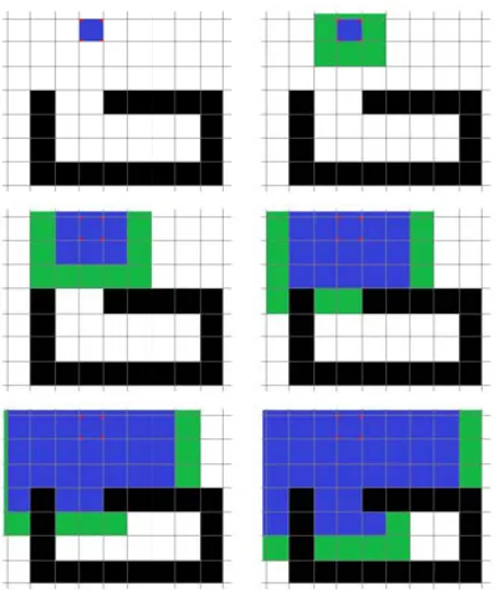
Figure 1 shows the definition of the terminology used
in this paper. In particular, the wavefront is defined as the cells that have not been given a global cost value, but have at least one neighbour with a global cost. This algo- rithm assumes each cell has eight neighbours and hence includes the diagonal neighbours in each calculation. This means on the subsequent iteration of the algorithm every cell in the wavefront will have a global cost calcu- lated for it and become “classified”.
For a grid containing n × n cells this algorithm will need to run a calculation for each cell, meaning an O(n2)
run time from a traditional sequential point of view, let alone the overhead of maintaining an ordered priority queue of yet to be visited paths. The concurrent algori- thm does not require any supporting data structures.
Figure 1. Definition of different classification of cells. Black represents a non-traversable grid square (obstacle), blue represents a classified traversable region, green represents the wave front about to be evaluated/classified, and white represents the unknown/unclassified region. The figure shows the progression of the wave front through the first five it- erations of the algorithm.
If the cost of traversal between cells is a uniform cost then the optimal cost value for each of these first genera- tion neighbouring cells can equally be based on the value of the original destination cell. In a two dimensional grid this means eight separate disjoint calculation steps. In a GPU these calculations can be done concurrently, thus using one iteration of the process rather than eight. In the subsequent wave front a sequential algorithm would re- quire sixteen cell calculations, which can also be done concurrently on a GPU. Table 2 shows how this number
of “iterations” increases at different rates for sequential and parallel solutions.
This reinforces the fact that from a theoretical point of view the traditional sequential algorithm runs in O(n2)
time whereas the proposed parallel algorithm runs in O(n) time.4
In theory, for uniform local cost environments it would be optimal if the cost calculation for a cell could only be run on a cell once. In practice, this is not possible without
Table 2. Comparison of cycles for sequential and parallel based algorithms.
Calculation per Wave Front
# .alcsC ∑ cycles (seq) ∑ cycles (||)
1 8 8 1
2 16 24 2
3 24 48 3
4 32 80 4
5 40 120 5
6 48 168 6
... ... ... ...
having to do some per-cell calculation in the kernel to determine whether the calculation should be done, which can be inefficient for large n.
The kernel makes the most significant progress when it is applied to cells in the wavefront. Therefore, a larger wave front will enable more cells to be calculated con- currently in one iteration. In practice wide open spaces in the occupancy grid promote larger wave fronts, while corridors limit wavefront growth. In an optimal best case where there are no obstacles an n × n grid can be comple- tely evaluated in n/
2 steps, that is, O(n) time. In the worst
case of a single cell wide corridor, the algorithm runs equally as slow as the sequential algorithm. As seen in the Experimental Results section the algorithm runs clo- ser to O(n) time than O(n2) in practice for environments a
field robot would be expected to traverse.
4.2. Implementation
The parallel algorithm was implemented using Open GL’s Shading Language (GLSL) [23]. Other mainstream programming languages such as nVidia’s CUDA [24], ATI’s Stream [25] and the generic successor OpenCL [26] were considered, but the grid based nature of an oc- cupancy grid intuitively maps to the texture-kernel pa- radigm associated with traditional graphical applications.
In most path planning algorithms mentioned in the Lit- erature Review section, unclassified cells are given the value of infinity to allow the algorithm to update the cell’s value given any initial finite calculation. In practice, this algorithm defines unclassified cells as having a value of –1. This value was chosen to represent unclassified cells for possible forward compatibility with stencil buf- fer operations (see the Future Work section). Obstacle cells are stored as –0.5. Negative numbers are used for determining special cells as normal classified cells will have a global finite cost greater than or equal to zero.
4.3. Multiple Destination Point Optimisation
4As stated in the Background section, in practice this may be hindered
by the number of processors available on the hardware. As graphics card manufacturers continue to increase the number of processors in GPUs this algorithm will tend towards linear execution time in prac-tice.
[image:4.595.304.541.111.221.2]make use of more processors in a single algorithm itera- tion. When working with multiple agents, there may be a situation where one or more agents are required to travel to more than one destination, where each destination has equal weight of importance. This scenario greatly bene- fits from the parallel implementation by providing multi- ple wave fronts and hence more grid cells situated in the wave front state every iteration.
4.4. Optimisation of Calculation using Expanding Texture
In the textbook definition of the ping-pong method the entire texture is requested to be rendered/evaluated every iteration. In the early stages of this algorithm there are many unclassified cells that are a large distance from the wave front that can be given to the shader pipeline if the entire texture (occupancy grid) is rendered every frame to iterate the algorithm.
One rough method to speed up the process is to render a sub-area of the texture as large as the wave front could possibly be at a given iteration of the calculation. Under this method, the sub-texture requested to be rendered gradually increases in size for each iteration of the algo-rithm. This technique is shown in Figure 2. Any texture
cell not rendered will be left in its prior state, and hence will not change. It should be noted that this only applies for single destination cases.
[image:5.595.311.533.395.542.2]As an example, in the very first iteration all eight of the destination’s neighbours will be evaluated. Therefore, the wave front will never be further than one cell from the destination and therefore no other cells are required to be given to a shader program for evaluation for this iteration. In short, at each stage, the area of the texture
Figure 2. The first four iterations of the algorithm. The red outline represents the size of the expanding texture re- quested to be evaluated/rendered by the GPU each itera- tion.
that is requested to be rendered gradually grows with the wavefront, so that (in the early generations) many of the redundant calculations of cells away from the wave front are not even considered. This is not perfect, as seen in the fourth iteration in Figure 2, as cells immediately behind
an obstacle are within the expanding texture’s bounds, but are still run through a shader program. Figure 3 shows
the execution time difference with and without expanding textures for an indoor environment of similar complexity to the L205 Office experiment detailed later in this paper. Using the expanding textures method of evaluation cuts the total number of calculations down by an order of magnitude. For environments with uniform local cost of traversability between cells, this method still has a high level of redundancy, as cells closer to the middle of the expanding texture will be evaluated to the same value many times. Using a stencil buffer to limit evaluation to only wave front cells is mentioned in Future Work.
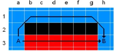
However, for a non-uniform environment, revaluation of cells not on the edge of the expanding texture is re-quired for correcting cells with differing traversal costs. In particular, this applies for paths that are spatially lon- ger (take up more cells) but have a lower cost due to effi- cient traversal between cells. Figure 4 shows a contrived
[image:5.595.60.286.494.670.2]example of this situation.
Figure 3. Comparison of execution time with and without expanding textures.
[image:5.595.329.515.585.668.2]Figure 4 shows two possible paths from A to B. Given
the cost of traversal Ct between two cells, x and y, with
local costs Cl(x) and Cl(y) can be given by the following
equation:
,
1 22
t l l
c c
C f C x C y k (2) where k = 1 for horizontal and vertical neighbours and k = √2 for diagonal neighbours, then the cost of the upper and lower paths is summarised in Table 3.
If the algorithm starts executing at B and begins to expand, at the seventh iteration it will first give cell A a global cost of 13.000. The wavefront that happens to be gradually evaluating the upper path will have just classi- fied cell b1 in the seventh iteration. Two iterations later, the algorithm will re-evaluate cell a3 and give it the more favourable value of 9.828. Unlike traditional path plann- ing algorithms, which expand based on lowest cost first, this algorithm expands on proximity or closest cell first, regardless of cost.
The inefficient re-evaluation of cell values due to an implementation limitation helps the more efficient wave fronts “wash over” already classified cells to make the resulting cost-to-go function more accurate. In Figure 4
this can also be seen in cell b3. As the algorithm evalu-ates the lower path, b3 is initially given a global cost of 11.5 from cell c3. When the upper path wave front even- tually “washes around” the obstacle from cell a2 it gives cell b3 a better global cost of 10.949. A cost-to-go func- tion is said to be mature if each cell had reached its final optimal value. Until the more efficient, but spatially longer, wave fronts wash over their sub-optimal counter- parts the function is considered immature.
4.5. Reading Values from Graphics Hardware
Current consumer graphics card hardware can have a large bottleneck in reading texture data back from graph- ics memory into the main memory used by the CPU rela- tive to algorithm execution time. The initial intension of this algorithm from a practical context was to make an identical function interface to the existing sequential al- gorithm so that there would be no modification to the other components of the system. That is, from an out-sider’s view, both CPU and GPU based versions of the exhaustive cost-to-go evaluation would take in an occu- pancy grid, a local traversal cost grid and a destination
Table 3. Comparison of lower and upper path options with differing traversal costs.
Path Cost (3d.p.) Number of cells
upper 9.828 9
lower 13.000 7
cell and fill out the traversable regions of the grid with global cost-to-go values. As a result, in the CPU based implementation, the entire grid evaluation for further path planning is provided ready of planning in CPU acce- ssible RAM. Although, internally, the evaluation step on a GPU is at least an order of magnitude better than the CPU version, the upload of values from graphical mem- ory to main memory provided a bottleneck that can, on some systems, nullify the GPU benefit.
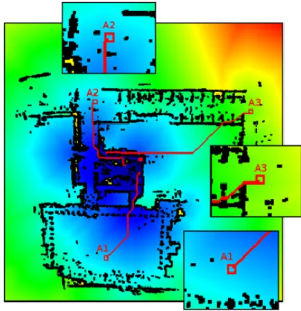
In practice, however, only the immediate area around an agent is required at any one time for path planning to occur. That is, even though a complete agent to destina- tion evaluation is required to properly plan on a global scale, the short term values of the evaluated traversability grid can be used to plan a local immediate path. For ex-ample, Figure 5 shows how three agents plan a path to a
common destination. Although the complete path from each agent to destination is calculated, it is only practical (even more so in dynamic environments) to decide upon a short term path. Therefore, only a small subregion of the cost-to-go function needs to be transferred back from GPU to CPU memory, as shown in the insets.
[image:6.595.56.287.675.718.2]This removes the burden imposed by the hardware bottleneck while still allowing the GPU to evaluate an exhaustive cost-to-go function efficiently.5
Figure 5. Example of multiple agents planning paths to a common destination on campus. Even though the cost-to-go function needs to be globally evaluated from the destination, only a small immediate region around the agent is required at any instant to do short term path planning.
5Of course, as graphics and motherboard hardware improves in terms
4.6. Algorithm Termination
Depending on the density of obstacles in the environment and layout of traversable paths for the evaluation wave front to travel through, the algorithm can take a different number of iterations before it generates a complete cost- to-go of the entire grid, or at least a required sub grid. For example, an environment with a low proportion of obstacles will allow the algorithm to spread quickly. On the other hand, a spiral or snaking corridor arrangement will force more iterations as less cells are being evaluated each iteration.
Knowing when to terminate the algorithm is important for practical applications as you may want to have an ex- haustive solution without having to do more calculations than required. The easiest approach is to look at the state space being evaluated and arbitrarily decide on a fixed number of iterations that would guarantee exhaustive eva- luation. For example, for an n × n grid, choosing an itera- tion count of a nominal value like 5n would work, but will result in redundant calculations being done on envi- ronments with open spaces. The advantage of this method, however, is that there is no overhead in determining algo- rithm termination.
An alternate method of measuring the progression of the algorithm is to calculate either the maximum or sum of the differences of all cells between step k – 1 and k. That is, if
1
where k k
x C x C x
(3) then the wavefront is still progressing into previously unclassified cells. From an implementation point of view, this condition can be applied to the entire grid via either of the following conditions of termination:
1 0
k i k i
i C x C x
(4)
1max Ck xi C xk i
0 (5) Both sum and maximum methods can theoretically run inO(1) + O(log4n) time,6 although the maximum method
provides more numerical stability on hardware that does not meet the full 32-bit floating point specification.7 Like
the minimum cell value method mentioned above, this can also be run periodically to reduce overhead on exe- cution time.
For environments that are explored and developed at a
slow rate a hybrid method can be utilised. Such a method would periodically use a maximum of differences algori- thm to check on the state for one complete evaluation. The number of algorithm iterations to complete this eva- luation can then be stored and assumed as a set value for a number of cycles, as previously discussed in the arbitr- ary value method.
The algorithm could also potentially be terminated ear- ly by monitoring the cell an agent resides in or monitor- ing a user defined set of cells or subregions, which inclu- de an agent’s cell. When the subregion’s cells all contain non-negative values, a path exists from the subregion to the destination cell. This path may not be the optimal path, but under some circumstances it could be close enough to optimal for practical purposes. Of course, if the agent does not have a valid path to the destination then the al- gorithm would still need to terminate based on a second- dary condition.
5. Experimental Results
The concurrent algorithm was applied to both simulated and real world environments to test both extreme cases and average operational cases, respectively. To test true practical benefit against an existing sequential algorithm, the execution or completion time of each test includes sending the occupancy grid data from CPU memory to graphical memory, performing the algorithm and copying a small portion of the texture back from graphical mem-ory to perform CPU based path planning on.8 Images of
the cost-to-go in the following experiments were gener- ated via a CPU based simulator. Real GPU benchmarks were done in two stages. The first stage used an on board laptop graphics card (ATI Radeon HD 2400 XT) for mo- re realistic test of practical applications. The second stage used a high end desktop graphics card (nVidia GeForce GTX 480) to show future potential of on board systems as well as potential live off board execution time.
The bench marked times are an approximation of the execution of one completion of the algorithm for a single occupancy grid as mentioned above. There is an inherent setup9 and shutdown time involved in executing the pro-
gram, which should not be included in the timing of the completion of the algorithm. Therefore, the following formula was used to estimate the single completion of the algorithm.
setup 512completions shutdown 512
T (6)
6Calculating the individual differences can run in a theoretical O(1)
time, followed by a Ping-Pong type reduction running in O(log4n) time
for the sum or maximum methods.
7Given an environment with global values ranging roughly from 0 to
1000, the maximum method will only need to keep track of numbers in the range 0 to 1000, whereas the sum method could potentially be handling much larger numbers than can be stored on a specific piece of graphics hardware [27].
8Path planning was not included in the experiment.
9Setup time includes acquiring a render context, compiling and linking
Each two-dimensional occupancy grid is generated from a three-dimensional laser range scan, fused with pose data derived from other sensor devices. Details of this config- uration can be found in [2]. Figure 6 shows the three-
dimensional point cloud data overlaid on the subsequen- tly real-time generated black and white occupancy grid. A video of this process running in real time can be found in [28]. The following sections outline a sample of the ex- periments run.
5.1. UNSW Middle Campus
This experiment was initially run under a CPU based si- mulator, where exhaustive evaluation was achieved in 370 wavefront progressions. Figure 7 shows the original
[image:8.595.58.286.277.435.2]occupancy grid generated from point cloud data. Figure
Figure 6. Real-time point cloud data overlaid on a real-time generated occupancy grid. Colours red through green are used to represent the spherical range of a point from the scanner itself. The occupancy grid uses darker colours to represent unexplored and traversable areas and lighter colours to represent obstacles.
Figure 7. Subsection of the original occupancy grid gener-ated from point cloud data. White represents obstacles. Black represents unknown/unexplored areas. Grey repre-sents areas that are known to be traversable.
8 shows the mature cost-to-go function. Table 4 shows
the bench marked times of the algorithm calculating a sin- gle exhaustive mature cost-to-go function on both the lap- top and desktop machines. A video of the algorithm run- ning in the CPU based simulator can be found with [28].
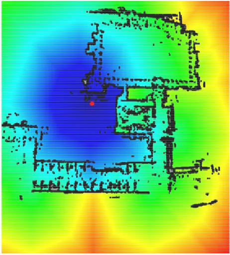
5.2. L205 Office
Under the CPU based simulator this occupancy grid achi- eved exhaustive evaluation in 1118 iterations. Figure 9
shows the mature cost-to-go function from the simulator output. Table 5 shows the bench marked times of the
algorithm calculating a mature cost-to-go function. The grid labelled normal sized denotes the original level of detail available from sensor processing to generate an oc- cupancy grid. However, this would provide grid cells be- tween 2.5 cm and 3.0 cm, which is more than enough for our UGVs. A quarter sized resolution occupancy grid was produced for benchmarking as it better matches the occu- pancy grid granularity required by our robots for success- ful navigation.10 The algorithm can be seen applied to the
[image:8.595.308.539.362.618.2]normal sized grid in [28].
Figure 8. Cost-to-go function applied to an occupancy grid generated from an Unmanned Ground Vehicle (UGV) being tele-operated around middle campus of UNSW. The grid represents an area of approximately 300 m × 300 m and uses 1024 × 1024 grid cells, resulting in an approximate grid size of 30 cm. Black pixels represent obstacles, indigo to red pixels represent increasing global cost and the red dot represents the destination location.
[image:8.595.59.288.514.673.2]Figure 9. Cost-to-go function applied to a hybrid technical drawing and post-processed occupancy grid of the layout of walls and large in obstacles the ME-L205 office at UNSW. The grid represents an area of approximately 33 m × 22 m and uses 1099 × 731 grid cells, resulting in an approximate grid size of 2.5 cm to 3 cm. As before, black pixels represent obstacles, indigo to red pixels represent increasing global cost and the red dot represents the destination location. Grey regions represent areas that are unreachable from the destination location and have hence remained unclassified.
Table 4. Comparison of the execution time of the parallel algorithm on different machines.
On Board Laptop Desktop
s
[image:9.595.57.286.462.500.2]4.498 s0.0478
Table 5. Comparison of the execution time of the parallel algorithm on different machines for normal and quarter sized occupancy grids.
Size On Board Laptop Desktop
Normal Size 11.113 ss 0.0580
Quarter Size 0.714 ss 0.0362
6. Future Work
The next step of this research will be to see if the stencil or depth buffer can be used to cull already classified cells within the bounds of the expanding texture at the current iteration. This would then enable the kernel to only be evaluated on cells in the wave front rather than those simply within the expanding texture. The stencil buffer is traditionally used to render pixels to screen that pass a stencil test. The test is based on a per-pixel value in the stencil buffer and is optimised to run outside the kernel execution in hardware.
Another direction this work is heading in is to expand the algorithm to a third dimension so that non-holonomic path planning can be done with, for example, (x, y, θ) like co-ordinates. It is also under investigation whether higher dimensional problems can be mapped to a two- dimensional equivalent for use in the proposed algorithm.
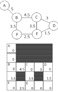
For this to happen, an efficient algorithm is to be invest- tigated that can map an undirected weighted graph to the grid structure for efficient cost generation. As a preview of the work Figure 10 shows how a given graph can be
mapped to “channels” in a grid structure for evaluation as a traditional occupancy grid. The channel approach en- forces one path between nodes that are connected in the original graph, but limits the number of paths from each node to four. If a node is more than degree four it can be split into two or more virtual nodes connected by zero cost channels.
A CUDA [24] implementation will also be investiga- ted from an implementation point of view, however the core algorithm will remain the same.
7. Conclusions
This paper presented a parallel implementation of a com- mon sequential algorithm in the field of path planning us- ing dynamic programming techniques. It provides an order of magnitude improvement on computation time for parti- cularly bad cases and many orders of magnitude for low obstacle density environments. In practice the implemen- tation has provided an option that remains real-time re- sponsive while allowing for the additional option of ei- ther larger traversability grids, more responsive calcula- tion or more fine grained grid structures tending towards approximating continuous space.
8. Acknowledgements
The authors would like to thank Mark Whitty and Jayan-tha Katupitiya for their contributions to the UNSW Mech- atronics UGV project that enabled the proposed algorithm to be tested on a physical platform.
[image:9.595.364.482.489.677.2]REFERENCES
[1] G. McComb and M. Predko, “Robot Builder’s Bonanza,” 3rd Editon, McGraw-Hill, Boston, 2006, pp. 654-656. [2] M. Whitty, S. Cossell, K. S. Dang, J. Guivant and J. Ka-
tupitiya, “Autonomous Navigation Using a Real-Time 3D Point Cloud,” Australasian Conference on Robotics and Automation, Brisbane, December 2010.
[3] A. Robledo, J. Guivant and S. Cossell, “Pseudo Priority Queues for Real-Time Performance on Dynamic Pro- gramming Processes Applied to Path Planning,” Austral- asian Conference on Robotics and Automation, Brisbane, December 2010.
[4] A. Elfes, “Using Occupancy Grids for Mobile Robot Per- ception and Navigation,” Computer, Vol. 22, No. 6, June 1989, pp. 46-57. doi:10.1109/2.30720
[5] D. Patterson, “The Trouble with Multicore,” IEEE Spec-trum Magazine, Vol. 47, No. 7, July 2010.
[6] P. F. Gorder, “Multicore Processors for Science and En-gineering,” Computing in Science and Engineering, Vol. 9, No. 2, April 2007, pp. 3-7. doi:10.1109/MCSE.2007.35
[7] GPGPU, “GPGPU,” Accessed December 2010. http://gpgpu.org/about
[8] nVidia Corporation, “GeForce GTX 480,” accessed De-cember 2010.
http://www.nvidia.com/object/product_geforce_gtx_480_ us.html
[9] J. Fung and S. Mann, “Openvidia: Parallel GPU Com-puter Vision,” Proceedings of the 13th annual ACM In- ternational Conference on Multimedia, Singapore, No- vember 2005, pp. 849-852.
[10] G. R. Andrews, “Concurrent Programming: Principles and Practice,” The Benjamin/Cummings Publishing Company, 1991.
[11] K. Fatahalian, J. Sugerman and P. Hanrahan, “Understan- ding the Efficiency of GPU Algorithms for Matrix-Matrix Multiplication,” Proceedings of the ACM SIGRAPH/EU-
ROGRAHICS Conference on Graphics Hardware, Greno-
ble, August 2004, pp. 133-137.
[12] nVidia Corporation, “High Performance Computing— Supercomputing with Tesla GPUs,” accessed December 2010.
http://www.nvidia.com/object/tesla_computing_solutions. html
[13] M. Harris, “GPU Gems 2,” Addison-Wesley, April 2005. [14] L. Magni, G. De Nicolao, L. Magnani and R. Scattolini,
“A Stablizing Model-Based Predictive Control Algorithm for Nonlinear Systems,” Automatica, Vol. 37, No. 9, Sep-
tember 2001, pp. 1351-1362.
[15] Y. K. Hwang and N. Ahuja, “A Potential Field Approach to Path Planning,” IEEE Transactions on Robotics and Automation, Vol. 8, No. 1, May 1989, pp. 23-32.
doi:10.1109/70.127236
[16] J. Barraquand, B. Langlois and J.-C. Latombe, “Numeri- cal Potential Field Techniques for Robot Path Planning,”
IEEE Transactions on Systems, Man and Cybernetics, Vol. 22, No. 2, March 1992, pp. 224-241.
doi:10.1109/21.148426
[17] C. I. Connolly, J. B. Burns and R. Weiss, “Path Planning using Laplace’s Equation,” IEEE International Confer- ence on Robotics and Automation, Cincinnati, May 1990, pp. 2102-2106.
[18] E. W. Dijkstra, “A Note on Two Problems in Connexion with Graphs,” Numerische Mathematik, Vol. 1, No. 1, 1959, pp. 269-271. doi:10.1007/BF01386390
[19] S.-H. Suh and K. G. Shin, “A Variational Dynamic Pro-gramming Approach to Robot-Path Planning with a Dis-tance-Safety Criterion,” IEEE Journal of Robotics and Automation, Vol. 4, No. 3, June 1988, pp. 334-349.
doi:10.1109/56.794
[20] J. Bruce, M. Veloso, “Real-Time Randomized Path Plan- ning for Robot Navigation,” IEEE/RSJ International Con- ference on Intelligent Robots and Systems, Lausanne, December 2002, pp. 2383-2388.
[21] T. Furukawa, B. Lavis and H. F. Durrant-Whyte, “Parallel Grid-Based Recursive Bayesian Estimation using GPU for Real-Time Autonomous Navigation,” IEEE Interna- tional Conference on Robotics and Automation, Anchor- age, May 2010, pp. 316-321.
[22] R. Bellman, “The Theory of Dynamic Programming,” RAND Corporation, 1954.
[23] SGI, “OpenGL Shading Language,” Accessed February, 2011. http://www.opengl.org
[24] nVidia Corporation, “CUDA Zone,” Accessed February, 2011. http://www.nvidia.com/object/cuda_home_new.html [25] Advanced Micro Devices Inc, “ATI Stream Technology,”
Accessed February 2011. http://www.amd.com [26] Khronos Group, “OpenCL,” Accessed February 2011.
http://www.khronos.org/opencl/
[27] M. Harris, “Mapping Computational Concepts to GPUs,”
ACM SIGGRAPH, Los Angeles, July 2005.
[28] Mechatronics at UNSW, “UNSW Mechatronics YouTube Channel,” Accessed March 2011.