Abstract— Recently statistical reasoning and methods like Six
Sigma are finding increased application in healthcare studies. Six Sigma is a highly disciplined approach to decision making that helps focus on improving processes to make them as near perfect as possible. This is highly desirable in an environment where mistakes can cost lives. However, this is limited to improvements in hospital administration whereas there is an unearthed potential in a clinical environment other than just reducing cycle times. In this paper, the cumulative distribution function of Gaussian curve and error function are studied to prove that Six Sigma ensures a nearly flawless process. Clinical trials are made on 30 human volunteers to monitor physiological parameter and histograms drawn to analyze repeatability of medical device used in the measurement process. The objective is to apply statistical science to discuss variations in medical devices, with the ultimate goal of advancing public health.
Index Terms—Gaussian Curve, Health care, Human
physiological parameters, Six Sigma, Statistics in medicine
I. INTRODUCTION
Six Sigma techniques have been largely associated with industrial methods and often there is a doubt whether a valid analogue exists between industry and health care. Healthcare organizations today increasingly have to cope with demands for the reduction of medical errors, together with a parallel need to reduce costs. Six Sigma is a methodology that can, and has, lent itself to the healthcare industry by establishing a high standard for acceptable quality while still focusing on the bottom-line [2], [4]. It goes beyond "continuous improvement" programs to specific, measurable goals, with the emphasis on measuring, improving and reporting clinical outcomes. Commonly used applications of Six Sigma to healthcare lie in minimizing or eliminating delay, repeated encounters, errors
Manuscript received February 15, 2008.
Dipali Bansal is with the Electronics & Communication Engineering Department, Apeejay college of Engineering., Sohna, Gurgaon, India (phone: 91-9910122000; e-mail: dipali.bansal@ yahoo.co.in).
Munna Khan is with the Electrical Engineering Department, Jamia Millia Islamia (A Central University), New Delhi, India (e-mail: [email protected]).
Deepak Goel is with the Purchase Department, ECEL, Faridabad, Haryana, India (e-mail: [email protected]).
A. K.Salhan is working in the Instrumentation Department, Defence Institute of Physiology and Allied Sciences, DRDO, Delhi, India (e-mail: [email protected]).
and inappropriate procedures. It has lead to reductions in medical errors, improvements in clinical outcomes, increases in cost-savings, and better organizational buy-in to quality initiatives [8], [9], [12].
The challenges however lie in the fact that the routes followed in a manufacturing process are clearly defined, whereas those followed by health care providers depend on clinical judgements at various stages, which may complicate a rigorous analysis. All approaches require strong leadership, adopt algorithmic approaches to problem solving based around iterative improvement, and promote the participation of people in all parts of the system. In the context of health care, these perspectives imply that we should not expect to invent systems that work perfectly immediately but rather that a process of gradual improvement should be designed into them, with all stakeholders participating in the improvement process [7]. The key issue is not the number of errors but having a systematic process to identify the sources of error and drive them down [3], [5].
In this paper we describe the industrial approach of six sigma—and explore how the concepts relate to health care, by making clinical trials on 30 human volunteers for analyzing physiological parameter like body temperature.
II. SIX SIGMA FOUNDATION
A. The Gaussian Probability
Six Sigma is a statistical tool derived from the concepts based on standard normal Gaussian curve as shown in Fig. 1. In real time almost anything will vary if we measure it with precision. For example consider a simple measurement tool like a one foot long scale. All of them might appear exactly one foot long. But if tested in a Standard’s laboratory, using a standard measuring device, you might find that some scales are 0.96 feet long while others are actually 1.06 feet long. They average out to one feet length, but each scale varies a little. Statisticians describe patterns of these variations with a bell shaped normal or Gaussian curve. (Carl Frederick Gauss was the mathematician who first worked out the mathematics of variation in the early Nineteenth century.) If the items being measured vary in a continuous manner, then the pattern described by the bell-shaped curve is achieved. 68.26% of the variation falls within two standard deviations. In statistics, the
Statistical Analysis of Human Physiological
Parameter using Six Sigma Techniques
Greek letter sigma (σ) is used to denote one standard
deviation. 99.73% of all deviations fall within 6 standard deviations. In Fig. 1 we show three sigma to the right of the mean. Imagine that we subdivided the 0.13% of the curve out on the right and inserted three more sigma. In other words, we would have six sigma to the right of the mean, and some very small amount beyond that. In fact, we could cover 99.99966% of the deviation and only exclude 3.4 instances in a million . Six Sigma projects rely on formulas and tables to determine sigma [6]. The only point you need to remember is that we want to define what we mean by a defect, and then create a process that is so consistent that only 3.4 defects will occur in the course of one million instances of the process.
Fig.1 The bell shaped Gaussian normal curve
The Gaussian curve is being used for analysis because most of the events in real life are random and can be characterized using the bell shaped normal distribution statistics. Random variables having Gaussian probability density functions are called Gaussian random variables [11].
A Gaussian random variable X with mean mx , standard
deviation σx and variance σ2x has a probability density
function fx(x) given by
“(1)”
.∞
<
<
∞
−
=
⎥⎥⎦ ⎤ ⎢ ⎢ ⎣ ⎡ − −x
for
e
x
f
x x m x x x 2 2( )2 1
2
1
)
(
σσ
π
(1)
The corresponding cumulative distribution function F(x) of normal distribution curve given by “
(2)
” helps in analysing the statistics of 6σ where ‘σ’ is the standard deviation of the normal curve from the mean value ‘m’.dv
e
x
X
P
x
F
x vm
∫
∞ − ⎥ ⎥ ⎦ ⎤ ⎢ ⎢ ⎣ ⎡ − −=
≤
=
2 ) ( 2 2 12
1
)
(
)
(
σσ
π
(2)
In “(2)”, ‘v’ is a dummy variable used to evaluate F(x). The integral involved in “(2)”, cannot be evaluated easily because it cannot be expressed in terms of elementary functions. It is however, simplified using concepts of error function and its mathematical tabulated values, which otherwise is a tedious task.
B. Error Function
Error function for a random variable ‘u’ is written as erf(u) and is defined using “(3)”.
∫
−=
u zdz
e
u
erf
0 ) ( 22
)
(
π
(3) ‘z’ in “(3)”, is also a random variable. The cumulative distribution function given by “(2)” can be expressed in terms of error functions using simple manipulations done below in “(4)”, obtained by rewriting “(2)” .dv
e
dv
e
x
F
x m v m v∫
∫
∞ ∞ ∞ − ⎥ ⎥ ⎦ ⎤ ⎢ ⎢ ⎣ ⎡ − − ⎥ ⎥ ⎦ ⎤ ⎢ ⎢ ⎣ ⎡ − −−
=
2 ) ( 2 2 1 2 ) ( 2 2 12
1
2
1
)
(
σ σσ
π
σ
π
(4) The first integral on the right hand side of “(4)” is the integral evaluated from –
∞
to∞
for the probability density function (p.d.f) of fx(x). By the property for p.d.f :∫
∞∞
=
-x
(x)dx
1
f
(5)Using “(5)”, we obtain a simplified version of “(4)” as below.
dv
e
x
F
x m v∫
∞ ⎥ ⎥ ⎦ ⎤ ⎢ ⎢ ⎣ ⎡ − −−
=
2 ) ( 2 2 12
1
1
)
(
σσ
π
(6)Let
σ
2
m
v
t
=
−
⇒
σ
2
dv
dt
=
(7)Replacing set of equations from “(7)” into “(6)” we obtain modified F(x) as below:
dt
e
x
F
m x tσ
σ
π
σ2
2
1
1
)
(
2 2∫
∞ − ⎥⎦ ⎤ ⎢⎣ ⎡ −−
=
Or
F
x
e
dt
m x t
∫
∞ − ⎥⎦ ⎤ ⎢⎣ ⎡ −−
=
σπ
2 21
1
)
The complementary error function denoted as erfc(u), is related to the error function by the equation given below
)
(
1
)
(
u
erf
u
erfc
=
−
∫
∞ −=
⇒
u zdz
e
u
erfc
(
)
2
2π
(9)Modifying “(8)” in terms of erfc(u) by using “(9)” we have
⎥
⎥
⎥
⎦
⎤
⎢
⎢
⎢
⎣
⎡
−
=
∫
∞ − ⎥⎦ ⎤ ⎢⎣ ⎡ −dt
e
x
F
m x t σπ
2 22
2
1
1
)
(
⎥⎦
⎤
⎢⎣
⎡ −
−
=
σ
2
2
1
1
)
(
x
erfc
x
m
F
(10)⎥⎦
⎤
⎢⎣
⎡ −
+
=
σ
2
2
1
2
1
)
(
x
erf
x
m
F
(11)In general, for a mean m=0, the cumulative distribution function can be denoted as below:
⎥⎦
⎤
⎢⎣
⎡
+
=
σ
2
2
1
2
1
)
(
x
erf
x
F
(12)The error function and the complementary error function are useful in calculating probability associated with a random experiment having a Gaussian distribution. The probability that a random variable X is not away from a mean value mx by
an amount more than (k
σ
x), where k is a constant can be given by “(13)”.∫
+ −=
+
≤
≤
−
x xx x k m k m x x x
x
k
X
m
k
f
x
dx
m
P
σ
σ
σ
σ
)
(
)
(
(13)Or R.H.S
=
F
x(
m
x+
k
σ
x)
−
F
x(
m
x−
k
σ
x)
In terms of error function, the above equation can be written as
R.H.S
⎥
⎦
⎤
⎢
⎣
⎡
⎟
⎠
⎞
⎜
⎝
⎛−
−
⎟
⎠
⎞
⎜
⎝
⎛
=
2
2
2
1
k
erf
k
erf
The property for error function says ‘erf(u) = - erf(-u)’. Using this fact in the above equation we have the following:
⎥⎦
⎤
⎢⎣
⎡
=
+
≤
≤
−
2
)
(
m
k
X
m
k
erf
k
P
xσ
x xσ
x (14)For k=3 we have the probability as
997
.
0
2
3
)
3
3
(
=
⎥⎦
⎤
⎢⎣
⎡
=
+
≤
≤
−
X
m
erf
m
P
xσ
x xσ
x (15)Probabilities for various values of variance can thus be easily calculated using tabulated values of error function [10]. Error function details for different k values are in Table I, which is
derived from the ‘Area under the Normal (Gaussian) Curve’, tabulated data easily available in books for Higher Engineering Mathematics [1].
Thus, we can easily verify that a variance of 6-sigma has a probability of 0.997. In fact, 99.99966% of the deviation is covered and only 3.4 instances in a million is excluded – the concept of Six Sigma.
III. METHODOLOGY
Six Sigma implements a four phase methodology detailed below [4], [6], [13]:
Measure—Process is identified for defects that influence
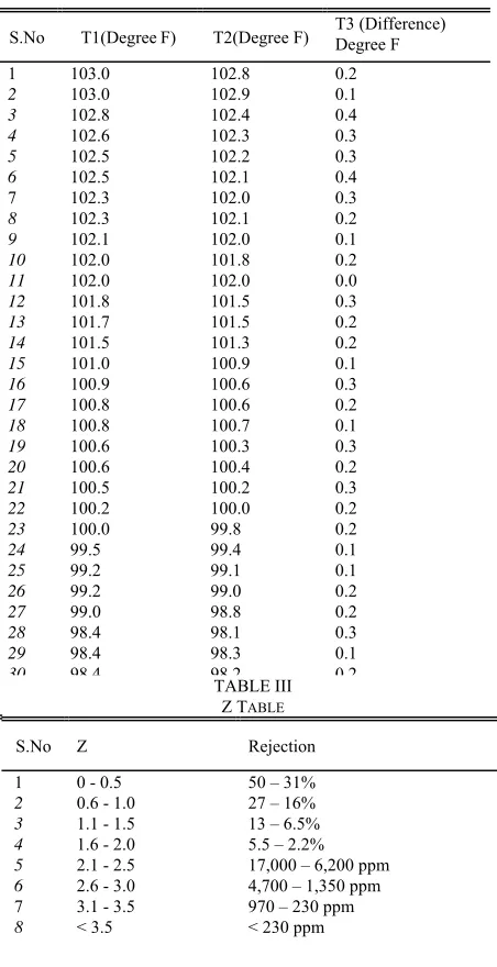
critical customer requirements and collected. Physiological data is measured on 30 human volunteers. Temperature is measured using two different Digital Thermometers of the same make for each subject and is recorded in Table II. T1 and T2 are Thermometer readings (in Degree Fahrenheit) obtained from two different meters.
Analyse—Differences are calculated for each subject for every
Thermometer reading and the variance is calculated. T3 is the difference in T1 and T2 in Degree Fahrenheit. Percentage rejection is estimated using the Z table in Table III and the formulae in “(16)”. Z table is obtained from standard Six Sigma calculation schemes where Z is the defect measurement error value. USL is the upper specification limit.
X
andσ
are the mean and standard deviation respectively.TABLE I
PROBABILITY FOR DIFFERENT K VALUES
S.No k
P
(
m
x−
k
σ
x≤
X
≤
m
x+
k
σ
x)
1 0.5 0.383
2 1.0 0.683 3 1.5 0.866 4 2.0 0.955 5 2.5 0.988
6 3.0 0.997 7 3.5 0.9995
⎟⎟
⎠
⎞
⎜⎜
⎝
⎛
−
=
σ
X
USL
Z
(16)
Improve—The impact of these variables are quantified and
acceptable ranges determined—one sigma, two sigma, three sigma etc. Histogram is drawn for the difference in temperature and then deviation is calculated from the Gaussian curve obtained using Mini Tab. Mini Tab is the application software used for statistical analysis using Six Sigma techniques.
Control—Process performance is monitored using statistical
process control tools. The results can be used to calibrate the medical devices and thus improve their quality.
TABLE II
THERMOMETER READINGS IN DEGREE FAHRENHEIT
IV. RESULTS AND DISCUSSIONS
[image:4.612.54.280.284.724.2]The Histogram plot for variation in temperature readings obtained using two thermometers of same make is in Fig.2. As can be seen, the mean of 30 recordings made, comes out to be 0.21. The standard deviation calculated is 0.09595. Using “(16)” and assuming USL=0.3, the calculated value of Z=3.12. From the standard Z-table, the corresponding rejection percentage comes out to be equal to 970 ppm.
Fig.2 The Histogram plot for variation in temperature readings obtained using two thermometers of same make.
The observations and analysis is purely based on comparison of temperature readings of two Thermometers. The variation has not been studied against any standard calibrated instrument from an accredited institution. The defect rates has been calculated with an assumption of USL = 0.3. The defect rates can also be studied for various values of USL.
Similar variance analysis is possible for a host of clinical instruments and processes. The results can throw clear scope of improvement in the process and would lead to better clinical analysis and possibly reduced iterations in treatment. All this opens up an avenue for waste reduction and cost savings in the process.
V. CONCLUSIONS
The Medical Devices should be user friendly and accurate as well, because even small variation in measurements can lead to wrong conclusions during clinical analysis. There may always be a gap between demand and supply of quality and trained managers, doctors and technicians, better approach definitely lies in tracing cause for variances and establishing reliable processes and end products. This would ensure that the normal health care can be naturally established and reach the masses. Historical quality assurance programs do not appear to be significantly improving the total testing and recording process.
S.No T1(DegreeF) T2(Degree F) T3 (Difference) Degree F
1 103.0 102.8 0.2
2 103.0 102.9 0.1
3 102.8 102.4 0.4
4 102.6 102.3 0.3
5 102.5 102.2 0.3
6 102.5 102.1 0.4
7 102.3 102.0 0.3
8 102.3 102.1 0.2
9 102.1 102.0 0.1
10 102.0 101.8 0.2
11 102.0 102.0 0.0
12 101.8 101.5 0.3
13 101.7 101.5 0.2
14 101.5 101.3 0.2
15 101.0 100.9 0.1
16 100.9 100.6 0.3
17 100.8 100.6 0.2
18 100.8 100.7 0.1
19 100.6 100.3 0.3
20 100.6 100.4 0.2
21 100.5 100.2 0.3
22 100.2 100.0 0.2
23 100.0 99.8 0.2
24 99.5 99.4 0.1
25 99.2 99.1 0.1
26 99.2 99.0 0.2
27 99.0 98.8 0.2
28 98.4 98.1 0.3
29 98.4 98.3 0.1
30 98.4 98.2 TABLE III 0.2
Z TABLE
S.No Z Rejection
1 0 - 0.5 50 – 31%
2 0.6 - 1.0 27 – 16% 3 1.1 - 1.5 13 – 6.5% 4 1.6 - 2.0 5.5 – 2.2% 5 2.1 - 2.5 17,000 – 6,200 ppm
6 2.6 - 3.0 4,700 – 1,350 ppm 7 3.1 - 3.5 970 – 230 ppm
Quality system solutions for performance improvement like Six Sigma may provide a systematic approach to improving medical equipment performance and would automatically ensure better, fast and reduced cost of treatments. Application of Six Sigma should be enriched in clinical research in terms of Medical Instrumentation improvements and standardization. Clearly this opens a whole spectrum of application of statistical techniques like Six Sigma and derived concepts like lean not only in improving customer satisfaction through better medical administration but making an impact on reliable clinical analysis and overall quality of medical care.
REFERENCES
[1] B.S.Grewal, “Higher Engineering Mathematics”, 36th edition, July 2001.
[2] Business process trends newsletter, “Six sigma today”, Volume 1, no. 6, June 2003.
[3] C.M. Creveling, J.L. Slutsky, D. Antis, “Design for Six Sigma: In Technology and Product Development”, Prentice Hall, 2003. ISBN 0-13-0092231.
[4] Greg Brue, “Six Sigma for Managers”, Tata McGraw-Hill, Edition 2002. [5] Joseph A. De Feo, William W Barnard, “JURAN Institute's Six Sigma Breakthrough and Beyond - Quality Performance Breakthrough
Methods”, Tata McGraw-Hill Publishing Company Limited, 2005, ISBN 0-07-059881-9.
[6] Matt Barney, Tom McCarty, “The New Six Sigma”, Motorola University, Prentice Hall, 2003.
[7] Mikel Harry, Richard Schroeder, “Six Sigma”, Random House, Inc, 2000, ISBN 0-385-49437-8.
[8] Nevalainen D, Berte L, Kraft C, Leigh E, Picaso L, Morgan T, “Evaluating laboratory performance on quality indicators with the six sigma scale”, PMID: 10747306.
[9] Novis DA, Jones BA, “Interinstitutional comparison of bedside blood glucose monitoring program characteristics, accuracy performance, and quality control documentation, PMID: 9625416.
[10] P.Chakrabarti, “A Text Book of Analog & Digital Communication”, Dhanpat Rai & Co. Edition 2006.
[11] R. P. Singh, S. D. Sapre, “Communication Systems – Analog and Digital”, Tata McGraw-Hill Publishing Company Limited, New Delhi, 26th reprint 2006.
[12] Terry Young, Sally Brailsford, Con Connell, Ruth Davies, Paul Harper, Jonathan H Klein, “Using industrial processes to improve patient care”, BMJ Publishing Group Ltd, 2004 January 17; 328(7432), pp.162–164. [13] Wheeler, Donald J, “The Six Sigma Practitioner's Guide to Data
Analysis”, p307, http://www.spcpress.com.