MAP estimators for piecewise continuous inversion

warwick.ac.uk/lib-publications

Original citation:

Dunlop, Matthew M. and Stuart, Andrew M.. (2016) MAP estimators for piecewise

continuous inversion. Inverse Problems, 32 (10). 105003.

Permanent WRAP URL:

http://wrap.warwick.ac.uk/79767

Copyright and reuse:

The Warwick Research Archive Portal (WRAP) makes this work of researchers of the

University of Warwick available open access under the following conditions.

This article is made available under the Creative Commons Attribution 3.0 (CC BY 3.0) license

and may be reused according to the conditions of the license. For more details see:

http://creativecommons.org/licenses/by/3.0/

A note on versions:

The version presented in WRAP is the published version, or, version of record, and may be

cited as it appears here.

This content has been downloaded from IOPscience. Please scroll down to see the full text.

Download details:

IP Address: 137.205.202.97

This content was downloaded on 16/12/2016 at 12:10 Please note that terms and conditions apply.

MAP estimators for piecewise continuous inversion

View the table of contents for this issue, or go to the journal homepage for more 2016 Inverse Problems 32 105003

(http://iopscience.iop.org/0266-5611/32/10/105003)

You may also be interested in:

Inverse Modeling: Functional analytic tools G Nakamura and R Potthast

Inverse Modeling: Analysis: uniqueness, stability and convergence questions G Nakamura and R Potthast

Well-posed Bayesian geometric inverse problems arising in subsurface flow Marco A Iglesias, Kui Lin and Andrew M Stuart

Bayesian approach to inverse problems for functions with a variable index Besov prior Junxiong Jia, Jigen Peng and Jinghuai Gao

A TV-Gaussian prior for infinite-dimensional Bayesian inverse problems and its numerical implementations

Zhewei Yao, Zixi Hu and Jinglai Li

Inverse problems with Poisson data: statistical regularization theory, applications and algorithms Thorsten Hohage and Frank Werner

Simultaneous reconstruction of the solution and the source of hyperbolic equations from boundary measurements: a robust numerical approach

Nicolae Cîndea and Arnaud Münch

A regularizing iterative ensemble Kalman method for PDE-constrained inverse problems Marco A Iglesias

MAP estimators for piecewise continuous

inversion

M M Dunlop

and A M Stuart

Mathematics Institute, University of Warwick, Coventry, CV4 7AL, UK

E-mail:[email protected]@warwick.ac.uk Received 10 September 2015, revised 14 June 2016

Accepted for publication 29 June 2016 Published 8 August 2016

Abstract

We study the inverse problem of estimating afielduafrom data comprising a

finite set of nonlinear functionals of ua, subject to additive noise; we denote this observed data by y. Our interest is in the reconstruction of piecewise continuous fields ua in which the discontinuity set is described by a finite number of geometric parametersa. Natural applications include groundwater

flow and electrical impedance tomography. We take a Bayesian approach, placing a prior distribution onuaand determining the conditional distribution onuagiven the datay. It is then natural to study maximuma posterior(MAP) estimators. Recently (Dashtiet al2013 Inverse Problems29 095017)it has been shown that MAP estimators can be characterised as minimisers of a generalised Onsager–Machlup functional, in the case where the prior measure is a Gaussian randomfield. We extend this theory to a more general class of prior distributions which allows for piecewise continuousfields. Specifically, the prior field is assumed to be piecewise Gaussian with random interfaces between the different Gaussians defined by afinite number of parameters. We also make connections with recent work on MAP estimators for linear pro-blems and possibly non-Gaussian priors (Helin and Burger 2015 Inverse

Problems 31 085009) which employs the notion of Fomin derivative. In

showing applicability of our theory we focus on the groundwaterflow and EIT models, though the theory holds more generally. Numerical experiments are implemented for the groundwaterflow model, demonstrating the feasibility of determining MAP estimators for these piecewise continuous models, but also that the geometric formulation can lead to multiple nearby (local)MAP esti-mators. We relate these MAP estimators to the behaviour of output from Inverse Problems32(2016)105003(50pp) doi:10.1088/0266-5611/32/10/105003

1

Author to whom any correspondence should be addressed.

Original content from this work may be used under the terms of theCreative Commons Attribution 3.0 licence. Any further distribution of this work must

maintain attribution to the author₍s₎and the title of the work, journal citation and DOI.

MCMC samples of the posterior, obtained using a state-of-the-art function space Metropolis–Hastings method.

Keywords: inverse problems, Bayesian approach, geometric priors, MAP estimators, EIT, groundwaterflow

(Somefigures may appear in colour only in the online journal)

1. Introduction

1.1. Context and literature review

A common inverse problem is that of estimating an unknown function from noisy mea-surements of a(possibly nonlinear)map applied to the function. Statistical and deterministic approaches to this problem have been considered extensively. In this paper we focus on the the study of MAP estimators within the Bayesian approach; these estimators provide a natural link between deterministic and statistical methods. In the Bayesian formulation, we describe the solution probabilistically and the distribution of the unknown, given the measurements and a prior model, is termed the posterior distribution. MAP estimators attempt to work with a notion of solutions of maximal probability under this posterior distribution and are typically characterised variationally, linking to deterministic methods.

There are two main approaches taken to the study of the posterior. The first is to discretise the space, and then apply finite dimensional Bayesian methodology [18]. An advantage to this approach is the availability of a Lebesgue density and a large amount of previous work which can then be built upon; but issues may arise (for example computa-tionally)when the dimension of the discretisation space is increased. An alternative approach is to apply infinite dimensional methodology directly on the original space, to derive algo-rithms, and then discretise to implement. This approach has been studied for linear problems in [12,25, 27], and more recently for nonlinear problems [10,21, 22,33]. It is the latter approach that we focus on in this paper.

In some situations it may be that point estimates are more desirable, or more computa-tionally feasible, than the entire posterior distribution. A detailed study of point estimates can be found in for example [24]. Three different estimates are commonly considered: the pos-terior mean which minimises L2loss, the posterior median which minimises L1 loss, and posterior modes which minimise zero-one loss. The former two estimates are unique[28], but a distribution may possess more than one mode. A consequence of this is that the posterior mean and median may be misleading in the case of a multi-modal posterior. Posterior modes are often termed maximum a posteriori(MAP)estimators in the literature.

In this paper we focus on MAP estimation. If the posterior has Lebesgue densityρ, MAP estimators are given by the global maxima ofρ. The problem of MAP estimation in this case is hence a deterministic variational problem, and has been well-studied[18]. In the infi nite-dimensional setting there is no Lebesgue density, but there has been recent research aimed at characterising the mode variationally and linking to the classical regularisation techniques described in, for example, [9]in the case when Gaussian priors are adopted. Non-Gaussian priors have also been considered in the infinite dimensional setting—in [14] weak MAP

In this paper we make a significant extension of the work in[9]to include priors which are defined by a combination of Gaussian random fields and a finite number of geometric parameters which define the different domains in which the different randomfields apply. We thereby study the reconstruction of piecewise continuous fields with interfaces defined by a

finite number of parameters. Our motivation for doing so comes from the work in[5], and its predecessors. In that paper a Bayesian inverse problem for piecewise constant fields, mod-elling the permeability appearing in a two-phase subsurface flow model, was studied. Such piecewise continuous fields were also previously studied in a groundwater flow context in

[16], where existence and well-posedness of the posterior distribution were shown. The idea of single point estimates being misleading is discussed and the existence of multiple local MAP estimators is shown. We also link our work to that in[14], by characterising the MAP estimator via the Fomin derivative.

Throughout this paper we focus on two model problems: groundwaterflow and electrical impedance tomography(EIT). Both of these problems are important examples of large scale inverse problems, with applications of great economic and societal value. MAP estimation in such problems has been studied previously[2,4,17,31]. However our formulation is quite general; for brevity we simply illustrate the theory for groundwater flow and EIT, and the numerics only in the case of groundwaterflow.

1.2. Mathematical setting

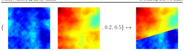
LetXbe a separable Banach space and letL Ík_{.Xshould be thought of as a function space} andΛa space of geometric parameters. Given(u a, )ÎX´ L, we construct another function

Î

ua Z_{, say. Considering the ingredients u and a in the construction of this function u}a separately will be useful in what follows. An example of such a construction is shown in

figure1.

Suppose we have a (typically nonlinear) forward operator :X´ L Y, where 

=

Y J_{. If(u,a)denotes the true input to our forward problem, we observe datayÎY given} by

 h

= +

y (u a, ) ,

for any positive definite AÎJ´J _{denote A} -A 1 2

∣·∣ ≔ ∣ · ∣the weighted norm onJ_{. Under} certain conditions, using a form of Bayes’theorem, we may writeμin the form

⎜ ⎟

⎛

⎝  ⎞⎠

m d , du a µexp -1 u a -y_G m u n a

2 , d d .

2

0 0

( ) ∣ ( ) ∣ ( ) ( )

The modes of the posterior distribution, termed MAP estimators, can be considered‘best guesses’for the state(u,a)given the data y. We now state rigorously what we mean by a MAP estimator forμ, as in[9]. Given(u a, )ÎX´ L, denote byB u ad( , )the ball of radius δcentred at(u,a).

Definition 1.1 (MAP estimator).For eachd>0, define

m

=

d d d

Î ´L

u ,a argmax B u a, . u a, X

( ) ( ( ))

( ) 1.0

0.8

0.6

0.4

0.2

0.0_{0.0 0.2 0.4 0.6 0.8 1.0 0.0 0.2 0.4 0.6 0.8 1.0 0.0 0.2 0.4 0.6 0.8 1.0 0.0 0.2 0.4 0.6 0.8 1.0} 1.0

0.8

0.6

0.4

0.2

0.0

1.0

0.8

0.6

0.4

0.2

0.0

1.0

0.8

0.6

0.4

0.2

0.0

Figure 2.Possible setsAicorresponding to example2.1.

1.0

0.8

0.6

0.4

0.2

0.0_{0.0 0.2 0.4 0.6 0.8 1.0} 0.8

0.6

0.4

0.2

0.0

0.0 0.2 0.4 0.6 0.8 1.0 0.0 0.2 0.4 0.6 0.8 1.0 0.0 0.2 0.4 0.6 0.8 1.0 0.8

0.6

0.4

0.2

0.0

0.8

0.6

0.4

0.2

0.0

1.0 1.0 1.0

Figure 3.Possible setsAi, corresponding to example2.2.

1.0

0.8

0.6

0.4

0.2

0.0_{0.0 0.2 0.4 0.6 0.8 1.0 0.0 0.2 0.4 0.6 0.8 1.0 0.0 0.2 0.4 0.6 0.8 1.0 0.0 0.2 0.4 0.6 0.8 1.0} 1.0

0.8

0.6

0.4

0.2

0.0

1.0

0.8

0.6

0.4

0.2

0.0

1.0

0.8

0.6

0.4

0.2

0.0

Any point( ¯ ¯)u a, ÎX´ L satisfying

m

m =

d

d d d d



B u a

B u a

lim ,

, 1

0

( ( ¯ ¯))

( ( ))

is called a MAP estimator for the measureμ.

If this definition is applied to probability measures defined via a Lebesgue density, MAP estimators coincide with maxima of this density. Here we extend the notion to the study of piecewise continuous fields.

1.3. Our contribution

The primary contributions of the paper are fourfold:

(i)We develop the MAP estimator theory for infinite dimensional geometric inverse problems involving discontinuousfields, building on theory in both of the recent papers

[9, 14], and opening up new avenues for the study of MAP estimators in infinite dimensional inverse problems.

(ii)We explicitly link MAP estimation for these geometric inverse problems to a variational Onsager–Machlup minimisation problem.

(iii)We show that the theory applies to the groundwaterflow model as in[16]and we show that the theory applies to the EIT problem as in [11].

(iv)We implement numerical experiments for the groundwaterflow model and demonstrate the feasibility of computing (local) MAP estimators within the geometric formulation, but also show that they can lead to multiple nearby solutions. We relate these multiple MAP estimators to the behaviour of output from MCMC to probe the posterior.

1.4. Structure of the paper

• In section2we describe the forward maps associated with the groundwaterflow and EIT problems, and show that they have the appropriate regularity needed in sections4–5.

• In section3we describe the choice of, and assumptions upon, the prior distribution whose samples comprise piecewise Gaussian randomfields with random interfaces.

• In section4we show existence and uniqueness of the posterior distribution.

• In section5 we define MAP estimators and prove their equivalence to minimisers of an appropriate Onsager–Machlup functional.

• In section6 we present numerics for the groundwaterflow problem. We consider three different prior models and investigate maximisers of the posterior distribution.

• In section7we conclude and outline possible future work in the area. 1.0

0.8

0.6

0.4

0.2

0.0

0.0 0.2 0.4 0.6 0.8 1.0 0.0 0.2 0.4 0.6 0.8 1.0 1.0

0.8

0.6

0.4

0.2

0.0

1.0

0.8

0.6

0.4

0.2

0.0

1.0

0.8

0.6

0.4

0.2

0.0

0.0 0.2 0.4 0.6 0.8 1.0 0.0 0.2 0.4 0.6 0.8 1.0

2. The forward problem

We consider two model problems. Our first problem (groundwater flow) is that of deter-mining the piecewise continuous permeability of a medium, given noisy measurements of water pressure(or hydraulic head)within it. The second problem (EIT)is determination of the piecewise continuous conductivity within a body from boundary voltage measurements. In what follows, thefinite dimensional spaceΛwill be a space of geometric parameters defining the interfaces between different media, andXwill be a product of function spaces defining the values of the permeabilities/conductivities between the interfaces.

We begin in section2.1by defining the construction map₍u a, ₎ua_{for the piecewise} continuous fields. In sections2.2and2.3we describe the models for groundwaterflow and EIT respectively, and prove regularity properties of the resulting forward maps; these prop-erties are required for our subsequent theory.

2.1. Defining the interfaces

LetDÍd _{be the domain of interest and letL Í}k_{be the space of geometric parameters.} Take a collection of set-valued maps Ai :L ( ),D i=1,K,Nsuch that for eacha Î L we have

Ç

= = Æ ¹

=

A a D, A a A a ifi j.

i N

i i j

1

⋃ ( ) ( ) ( )

We assume that each mapAiis continuous in the sense that

-   D 

a b 0 A ai A bi 0,

∣ ∣ ∣ ( ) ( )∣

where Δdenotes the symmetric difference:

È

A B≔ ( ⧹ )A B ( ⧹ )B A .

Let X=C0₍D;N_{). Given u= u,¼,u ÎX} N 1

( ) and a Î L we define the function

Î ¥

ua L _{( )}D _by

å

=

=



ua F u a, u . 2.1

i N

i A a 1

i

( ) ≔ ( ) ( )

Where F:X´ L L¥( )D is the construction map.

We give four examples of the functionsAiand the sets/interfaces they define.

Example 2.1. Let D=_[0, 1_]2_{,L =[0, 1]}2 _{and N=2. We specify points a and b on} either side of the square D and join them with a straight line. We then let A a b1( , ) be the

region of Dbelow this line and A a b2( , )=D A a b⧹ 1( , ). Example setsAi(a,b) for various parametersa,b are shown infigure2.

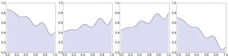
Example 2.2. Let D=_[0, 1_]2_{, L =[0, 1]}2 _{and N}=_{2. Choose a continuous map}

L  ¥

H: L ([0, 1])such thatH a b( , )( )0 =a andH a b( , )( )1 =bfor all(a b, )Î L. Let A a b1( , ) be the region of D beneath the graph of the curve H a b( , ) and let

=

A a b2( , ) D A a b⧹ 1( , ). This setup includes the previous example:

= +

-H a b x( , )( ) a (b a x) defines the appropriate straight lines. The continuity of A1and A2can be seen by noting that

 

ò

D = D

-- ¥

 

A a b A a b A a b A a b

H a b x H a b x x

H a b H a b

, , , ,

, , d

, ,

1 1 1 1 2 2 2 1 1 2 2 2

0 1

1 1 2 2

1 1 2 2

∣ ( ) ( )∣ ∣ ( ) ( )∣

∣ ( )( ) ( )( )∣

( ) ( )

and using the continuity of HintoL¥([0, 1]). For example, one may takeHto be given by

p

= + - +

H a b x( , )( ) a (b a x) xsin 6( x) 10

which can be seen to be continuous into L¥([0, 1]). Example sets Ai(a, b) for various parametersa,b, with this choice ofH, are shown infigure4.

Example 2.3. We can generalise the previous example to allow the inclusion of a fault. Let

=

D _[0, 1_]2_{, L =[0, 1]}2 _{´ -[ 1, 1] and N=2. Let pÎ(0, 1) denote the horizontal} location of the fault. Given H : 0, 1_{[ ]}2 L¥_([0, 1_{]) as in the previous example, define}

L  ¥

H˜ : L ([0, 1])by

⎧ ⎨ ⎩

= Î

+ Î

H a b c x H a b x x p

c H a b x x p

, , , 0,

, , 1

˜ ( )( ) ( )( ) [ ]

( )( ) ( ]

so that the parameter c determines the (signed) magnitude of the fault. Defining the sets A a b c1( , , ) and A a b c2( , , ) as the regions of D beneath and above the curve H a b c˜ ( , , ) respectively, the continuity can be seen in a similar manner to the previous example. Example sets Ai(a,b,c)for various parametersa,b,care shown in figure3.

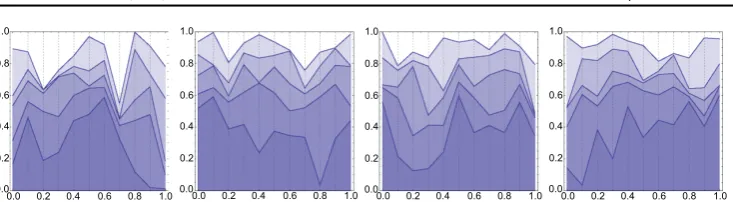
Example 2.4. Again working withD=_[0, 1_]2_{, but with a much larger parameter space,} one could also select points at specificx-coordinates and linearly interpolate between them. FixK N, Îand setL = XN- Í 0, 1 - ´

K N K

1 [ ]( 1) , whereXN-1is the simplex

   

XN-1={(y1,¼,yN-1)Î[0, 1]N-1∣0 y1 ¼ yN-1 1 .}

Then givena Î L, define the functionsfi(a),i=1,¼,N-1, to be the linear interpolation of

the points -

-=

a

,

j

K ij _j K 1

1 ₁

graphs of the functionsfi(a)and fi-1( ), anda =

È

-AN( )a D⧹ iN11 A ai( ). Example setsAi(a) for various parameters aare shown infigure5.

In order to see the continuity of these maps, wefirst partition the domain into stripsDj, ⎧

⎨ ⎩

⎫ ⎬ ⎭  

= Î

-- - = ¼

-D x y D j

K x

j

K j K

, 1

1 1 , 1, , 1

j ( )

so that we have

Ç

=

-A ai A a D.

j K

i j

1 1

( ) ⋃ ( )

It follows from properties of the symmetric difference that



_å

Ç

Ç

D D

=

-A ai A bi A a D A b D .

j K

i j i j

1 1

∣ ( ) ( )∣ ∣( ( ) ) ( ( ) )∣

It hence suffices to show that the maps Ai(·)

Ç

2.2. The Darcy model for groundwater flow

We consider the Darcy model for groundwater flow on a domainDÍd_{,d=1, 2, 3. Let} k=(kij) denote the permeability tensor of the medium, p the pressure of the water, and assume the viscosity of the water is constant. Darcy’s law [8]tells us that the velocity is proportional to the gradient of the pressure:

k

= - 

v p.

Additionally, a local form of mass conservation tells us that ·v=f.

Combining these two equations, and imposing Dirichlet boundary conditions for simplicity, results in the PDE

⎧ ⎨ ⎩

k

-  =

= ¶

p f D

p g D

in on .

· ( )

This is the PDE we will consider in the forward model, and it gives rise to a solution mapkp.

For simplicity we will work in the case where κis an isotropic (scalar) permeability, bounded above and below by positive constants, and so it can be represented as the image of some bounded function under a positive continuously differentiable maps:+.

LetV=H D1_{( ), the Sobolev space of once weakly differentiable functions on D[13].} Then given fÎH-1_{( ),}D _gÎ_H1 2₍¶_{D),u ÎXandaÎ L, definep ÎV}

u a, to be the solution of the weak form of the PDE

⎪

⎪

⎧ ⎨ ⎩

s

-  =

= ¶

u p f D

p g D

in

on . 2.2

a u a

u a

,

,

· ( ( ) )

( )

⎪

⎪

⎧ ⎨ ⎩

s s

-  = +  

= ¶

u q f u G D

q D

in

0 on . 2.3

a

u a a

u a

,

,

· ( ( ) ) · ( ( ) )

( )

The following lemma tells us that the map  is well defined and has certain regularity properties. Its proof is given in theappendix.

Lemma 2.5. The map:X´ L V is well-defined and satisfies:

(i)for each(u a, )ÎX´ L,

*

  + s ¥ k +

 (u a, )V ( f V  (ua)  L G V) min(u a, )  G V,

wherekmin(u a, )is given by

k = s >

Î

u a, essinf u x 0; x D

a min( ) ( ( ))

(ii)for each aÎ L,(·,a):XV is locally Lipschitz continuous, i.e. for everyr>0

there existsL r( )>0such that, for allu v, ÎX with u X, v X <rand alla Î L, we

have

 - 

- (u a, ) (v a, )V L r( )u vX;

(iii)for eachu ÎX,(u,·):L V is continuous.

We now choose a continuous linear observation operator ℓ:VJ_{. For example,} writingℓ=(ℓ1,¼,ℓJ), we could take

ò

= - - e = ¼

ℓ p 1 p y x i J

2 e d , 1, , 2.4

i

D d

x y 2

2

i 2 ( )

( ) ( ) ( )

∣ ∣

for somee>0, so thatℓiapproximates a point observation at the pointxiÎD. Our forward operator :X´ L J _{is then defined by=ℓ◦, so that it can be written as the} composition

k=s

   

u a, ua ua p ℓ p .

( ) ( ) ( )

From the above regularity ofwe can deduce the following regularity properties of our forward operator:

Proposition 2.6. Define the map:X´ L J_{as above. Then satisfies}

(i)For eachr>0 andu v, ÎX with u X, v X <r, there existsC r( )>0 such that for

allaÎ L,

 u a, - v a, C r u-vX.

∣ ( ) ( )∣ ( )

(ii)For eachu ÎX, the map₍u,_·):L J _{is continuous.}

Proof.

(i)The mapℓis defined to be a continuous linear functional, and so in particular is Lipschitz. Since we have=ℓ◦the result follows from lemma2.5(ii).

2.3. The complete electrode model(CEM)for EIT

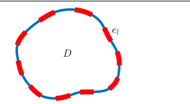
EIT is an imaging technique that aims to make inference about the internal conductivity of a body from surface voltage measurements. Electrodes are attached to the surface of the body, current is injected, and the resulting voltages on the electrodes are measured. Applications include both medical imaging, where the aim is to non-invasively detect internal abnormal-ities within a human patient, and subsurface imaging, where material properties of the sub-surface are differentiated via their conductivities. Early references include[15]in the context of medical imaging and[20]in the context of subsurface imaging.

The CEM is proposed for the forward model in [32], and shown to agree with exper-imental data up to measurement precision. In its strong form, the PDE reads

⎧

⎨ ⎪ ⎪ ⎪⎪

⎩ ⎪ ⎪ ⎪ ⎪

ò

k k k

k

-  = Î

¶

¶ = = ¼

¶

¶ = Î ¶

+ ¶

¶ = Î = ¼

=

x v x x D

v

n S I l L

x v

n x x D e

v x z x v

n x V x e l L

0

d 1, ,

0

, 1, , .

2.5

e l

l L

l

l l l

1

l

· ( ( ) ( ))

( ) ( ) ⧹ ⋃

( ) ( ) ( )

( )

The domain D represents the body, and ( )el lL=1Í ¶D the electrodes attached to its surface with corresponding contact impedances( )z_{l l}L₌₁. Figure6 shows an example domain and attached electrodes. A current Il is injected into each electrodeel, and a voltage mea-surementVlmade. Hereκrepresents the conductivity of the body, andvthe potential within it. Note that the solution comprises both a functionvÎH D1_{( )and a vector Î}

=

V_{l l}L L 1

( ) of

boundary voltage measurements.

A corresponding weak form exists, and is shown to have a unique solution (up to constants) given appropriate conditions on κ, ( )zl lL₌1 and ( )Il lL=1—see [32] for details. Moreover, under some additional assumptions, the mapping k( )Vl lL=1 is known to be Fréchet differentiable when we equip the conductivity space with the supremum norm[17]. We can apply different current stimulation patterns to the electrodes to yield additional information. Assume that we have M different (linearly independent) current stimulation patterns Im ₌

m M

1

( ( )) _{. This yieldsMdifferent mappingsk}

=

 V_lm l L

1

( ( )) each with the regularity above, or equivalently a mappingkV whereVÎJ _withJ=LM.

Analogously to the Darcy model case, we will consider isotropic conductivities of the formk=s₍ua_{), wheres:} _+_{is positive and continuously differentiable. Our forward} operator:X´ L J_{, is then given by the composition}

k=s ¼ ¼

   

u a, ua ua v1,V 1 , , vM,V M V 1, ,V M .

( ) ( ) (( ( ) ( )) ( ( ) ( ))) ( ( ) ( ))

We show in theappendixthat the map defined in this way has the same regularity as the map corresponding to the Darcy model.

Proposition 2.7. Define the map:X´ L J_{as above. Then satisfies}

(i)For eachr>0 andu v, ÎX with u X, v X <r, there existsC r( )>0 such that for

allaÎ L,

 u a, - v a, C r u-vX.

∣ ( ) ( )∣ ( )

3. Onsager–Machlup functionals and prior modelling

In this section we recall the definition of an Onsager–Machlup functional for a measure which is equivalent2 to a Gaussian measure. We then introduce the prior measures that we will consider,first on the function spaceX, then the geometric parameter spaceΛ, andfinally the product space X ´ L. We conclude the section by extending the definition of Onsager– Machlup functional so that it is appropriate for the measures we consider here, supported on

fields and geometric parameters which are combined to make piecewise continuous functions.

3.1. Onsager–Machlup functionals

The Onsager–Machlup functional of a measure is the negative logarithm of its Lebesgue density when such a density exists, and otherwise can be thought of analogously. We start by defining it precisely for measures defined via density with respect to a Gaussian, allowing for infinite dimensional spaces on which Lebesgue measure is not defined. Suppose thatμis a measure equivalent to a Gaussian measurem₀. Then the Onsager–Machlup functional forμis defined as follows.

Definition 3.1 (Onsager–Machlup functional I).Letμbe a measure on a Banach spaceZ

which is equivalent tom₀, wherem₀ is a Gaussian measure onZwith Cameron–Martin space

E. LetB zd( )denote the ball of radiusδcentred atzÎZ. A functionalI: Zis called the

Onsager–Machlup functionalforμif, for eachx y, ÎE,

m

m =

-d

d d



B x

B y I y I x

lim exp

0

( ( ))

( ( )) ( ( ) ( ))

and I x( ) = ¥for xÏE.

Remarks 3.2.

(i)The Onsager–Machlup functional is only defined up to addition of a constant.

(ii)If Z is finite dimensional and μ admits a positive Lebesgue density ρ, then

r

=

-I x( ) log ( )x for all xÎZ. In light of the previous remark, this is true even if ρ is not normalised.

(iii)LetZ=n_{befinite dimensional, and letm =N 0,S}

0 ( )be a Gaussian measure onZ. Let 

G Î m´m_{be a positive-definite matrix, AÎ}m´n_{and yÎ}m_{. Defineμby}

⎜ ⎟

⎛

⎝ ⎞⎠

m

m x µ - Ax-yG

d

d exp

1 2 0

2

( ) ∣ ∣

so that

⎜ ⎟

⎛

⎝ ⎞⎠

m

µ - - G - S

x x Ax y x

d

d exp

1 2

1

2 .

2 2

( ) ∣ ∣ ∣ ∣

Then by the previous remark, the Onsager–Machlup functional forμis given by

= - _G+ _S

I x 1 Ax y x

2

1 2

2 2

( ) ∣ ∣ ∣ ∣

for all xÎZ, which is a Tikhonov regularised least squares functional.

2

(iv)The preceding example(iii)may be extended to an infinite dimensional setting. LetZbe a separable Banach space, and let m₀=N(0,0) be a Gaussian measure on Z with Cameron–Martin space (E,⟨· ·⟩, E, · E). LetG Îm´m be a positive-definite matrix,





A: X m_{a bounded linear operator andyÎ}m_{. Defineμby}

⎜ ⎟

⎛

⎝ ⎞⎠

m

m x µ - Ax-yG

d

d exp

1

2 .

0

2

( ) ∣ ∣

Then theorem 3.2 in[9]tells us that the Onsager–Machlup functional forμis given by = - _G+  

I x 1 Ax y x

2

1 2 E.

2 2

( ) ∣ ∣

(iv)In this paper, the posterior distribution will be a measure on the product space

= ´ L

Z X . The prior distribution will be an independent product of a Gaussian onX

and a compactly supported measure onΛ. Due to the assumption of compact support, the prior will not be equivalent to a Gaussian measure onZand so the above definition does not apply; we provide a suitable extension to the definition in section3.4.

As we are taking a Bayesian approach to the inverse problem, we incorporate our prior beliefs about the permeability/conductivity into the model via probability measures onXand

Λ. We will combine these into a prior measure on the product spaceX´ L. We equip this space with any (complete) norm (· ·),  such that if (u a, ) 0, then  u X 0

and∣ ∣a 0.

3.2. Priors for the fields

We wish to put priors on the fieldsu1,¼,uN ÎC0( ). We use independent Gaussian mea-D sures ui~mi₀≔N m( i,i), where the means miÎC0( ), and each covariance operatorD i:C0( )D C0( )D is trace-class and positive definite. It follows that the vector

m m m

¼ ~ ´ ¼ ´

u1, ,uN ₀1 N₀ 0

( ) ≕ is Gaussian onX:

⎛ ⎝

⎜ ⎞

⎠ ⎟



m =

=

N m, ,

i N

i 0

1

⨁

wherem=(m1,¼,mN)ÎX. IfEidenotes the Cameron–Martin space[10]ofmi₀, then that of

m₀ is given by =

=

E E

i N

i 1

⨁

with inner product given by the sum of those of its component spaces. The Onsager–Machlup functional ofm₀ is known to be given by

⎪

⎪

⎧ ⎨ ⎩

= - - Î

¥ - Ï

 

J u u m u m E

u m E.

E 1

2

2

( )

This can be seen, for example, as a consequence of proposition 18.3 in[26].

correlations between the fields and the geometric parameters under the prior is a more technical issue however, and so we will assume that these are independent.

Example 3.4. Define the negative Laplacian with Neumann boundary conditions as follows:



ò

n

= -D = Î = ¶ =

A , A u H D du D u x x

d 0 on , D d 0 .

2

{

}

( ) ( )∣ ( )

ThenAis invertible. We can definei=A-ai, where eachai>d 2. Then eachiis trace-class and positive definite, and samples from eachmi₀will be almost surely continuous and so

m₀ can be considered as a Gaussian measure onX. Moreover, regularity of the samples will increase asaiincreases, see[10]for details.

3.3. Priors for the geometric parameters

We also want to put a prior measure on the geometric parameters, i.e. we want to choose a probability measure onΛ. SinceL Ík_{the analysis is more straightforward than the infinite} dimensional case. Let ν be a probability measure on Λ with compact supportSÍ L. We assumeνis absolutely continuous with respect to the Lebesgue measure and that its densityρ is continuous onS. Despite being defined on afinite dimensional space, the measureνis not necessarily equivalent to the Lebesgue measure on the whole of k and so the previous definition of Onsager–Machlup functional does not apply. We hence must formulate a new definition for this case.

Sincer>0onint( )S , we can use the continuity ofρto calculate the limits of ratios of small ball probabilities forν onint( )S . Leta a1, 2Îint( ), thenS

ò

ò

ò

ò

n n

r r

r r r

r

r r

=

=

=

=

-d

d

d _d

d

 



d

d

d _d

d _d

B a B a

a a

a a

a a

a a

a a

a a

lim lim

d

d

lim

d

d

exp log log .

B a

B a

B a _{B a}

B a _{B a} 0

1

2 0

0 1

1

1

2

1 2

1 2 1

1 2

2

( ( ))

( ( ))

( )

( )

( )

( )

( )

( )

( ( ) ( ))

( )

( )

∣ ( ) ∣ _{( )}

∣ ( ) ∣ _{( )}

If either a1ora2lie outside of Sthe limit can be seen to be 0 or¥respectively. It hence makes sense to define the Onsager–Machlup functional forνonL ¶⧹ S as

⎧ ⎨ ⎩

r

= - Î

¥ Ï

K a a a S

a S

log int

.

( ) ( ) ( )

ForaÎ ¶S, we defineK(a)to be the limit ofKfrom the interior:

r

= - Î ¶

 Î

K a lim log b a S

b a b intS

( ) ( )

( )

Remark 3.5. If we were to defineKon¶Sin the same way that we defined it onL ¶⧹ S,K

would have a positive jump at the boundary related to the geometry ofS. This would mean that K was not lower semi-continuous on S which would cause problems when seeking minimisers. The definition we have chosen is appropriate: if any minimising sequence

 Í an n 1 int S

( ) ( )of Khas an accumulation point on¶S, thenνhas a mode at that point. If we have no prior knowledge about the interfaces andΛis compact, we could place a uniform prior on the whole of Λ. Otherwise we could either choose a prior with smaller support, or one that weights certain areas more than others.

3.4. Priors on XΛ

We assume that the priors on thefields and the geometric parameters are independent, so that we may take the product measure m₀´n0 as our prior on X´ L. Note that if

´ L  ¥

F :X L ( )D denotes the construction map₍u a, ₎ua_{defined earlier by(2.1), then} our prior permeability/conductivity distribution on L¥( )D is given by the pushforward3

*

m =_F# m ´n

0 ( 0 0). This is much more cumbersome to deal with however, since for example

¥

L ( )D is not separable. It is for this reason we incorporate the mappingFinto the forward map . Assuming now that the prior m₀´n0 is as described above, we can define the Onsager–Machlup functional for measuresμonX´ Lwhich are equivalent tom₀´n0.

Definition 3.6 (Onsager–Machlup functional II).Letμbe a measure onX´ Lequivalent tom₀´n0, wherem₀andn0 satisfy the assumptions detailed above. LetB u ad( , )denote the ball of radius δ centred at (u a, )ÎX´ L. A functional I:X ´ L  is called the

Onsager–Machlup functionalforμif,

(i)for each(u a, ) (, v b, )ÎE´int( ),S

m

m =

-d d d



B u a

B v b I v b I u a

lim ,

, exp , , ;

0

( ( ))

( ( )) ( ( ) ( ))

(ii)for each(u a, )ÎE´ ¶S, =

 Î

I u a, lim I u b, ;

b a b intS

( ) ( )

( )

(iii)I u a( , )= ¥foru ÏE oraÏS.

4. Likelihood and posterior distribution

We return to the abstract setting mentioned in the introduction. LetXbe a separable Banach space,L Ík_andY=J_{. Suppose we have a forward operator:X´ L Y. If(u,a)} denotes the true input to our forward problem, we observe datayÎY given by

3

 h

= +

y (u a, ) ,

whereh~0≔N(0,G),G ÎJ´Jpositive definite, is Gaussian noise onYindependent of

the prior.

It is clear that we have y u a∣( , )~u a, ≔N( ( u a, ),G). We can use this to formally

find the distribution of(u a y, )∣ . First note that

⎜ ⎟

⎛

⎝ ⎞⎠

 dy =exp -F u a y, ; + 1 y_G  y

2 d ,

u a, ( ) ( ) ∣ ∣2 0( )

where the potential(or negative log-likelihood)F:X´ L ´Yis given by



F u a y, ; = 1 u a -y_G

2 , . 4.1

2

( ) ∣ ( ) ∣ ( )

Hence under suitable regularity conditions, Bayes’theorem tells us that the distributionμof u a y,

( )∣ satisfies

m(d , du a)µexp(-F(u a y, ; ))m₀(du)n0(da)

after absorbing theexp 1 y_G 2

2

(

)

We now make this statement rigorous. To keep the situation general, we do not insist that

Φ takes the form(4.1), and instead assert only thatΦsatisfies the following assumptions.

Assumptions 4.1. There existsX¢ ´ L¢ ÍX´ Lsuch that

(i)for everye>0 there is an M1( )e Îsuch that for alluÎ ¢X and allaÎ L¢

 e e

F(u a y, ; ) M1( )-  u 2X;

(ii)for eachuÎ ¢X and yÎY, the potentialF(u, ;· y):L¢ is continuous;

(iii)there exists a strictly positive M2:+´+´++ monotonic non-decreasing

separately in each argument, such that for eachr>0,uÎ ¢X anda Î L¢, andy y1, 2ÎY

with∣ ∣ ∣ ∣y1, y2 <r,



F u a y, ; ₁ - F u a y, ; ₂ M r2 , u X, a y1-y2;

∣ ( ) ( )∣ ( ∣ ∣)∣ ∣

(iv)there exists a strictly positive M3:+´ L ´Y+, continuous in its second component, such that for each r>0, aÎ L¢ and yÎY, and u u1, 2Î ¢X with

<

 u1 X, u2 X r,



F u a y1, ; - F u2, ;a y M r a y3 , , u1-u2X.

∣ ( ) ( )∣ ( )

These assumptions are used in the proof of existence and well-posedness of the posterior distribution, which is given in the appendix:

Theorem 4.2 (Existence and well-posedness). Let assumptions 4.1 hold. Assume that

m₀´n0 X¢ ´ L¢ =1

( )( ) , and that (m0´n0)((X¢ ´ L¢)

Ç

Í ´ L

B X . Then

(ii)for each yÎY,Z( )y given by

ò

= -F

´L

Z y exp u a y, ; du da

X 0 0

( ) ( ( )) ( ) ( )

is positive andfinite, and so the probability measuremy_,

m u a = -F m n

Z y u a y u a

d , d 1 exp , ; d d 4.2

y

0 0

( )

( ) ( ( )) ( ) ( ) ( )

is well-defined.

(iii)Assume additionally that, for everyfixedr>0, there existse>0with



e u +M r  u a ÎL_m´n X´ L

exp( X2)(1 2( , X,∣ ∣) )2 1₀ 0( ; ).

Then there isC r( )>0 such that for all y y, ¢ ÎY with∣ ∣ ∣ ∣y, y¢ <r,



m m ¢ - ¢

d y, y C y y .

Hell( ) ∣ ∣

Remark 4.3. In this paper we are focused on the case when thefield priorm₀is taken to be Gaussian. However, the above existence and well-posedness result still holds if, for example,

m₀ is taken to be Besov rather than Gaussian, since a Fernique-type theorem holds for such priors [10,23].

We show that for both choices of test models, the potential (4.1) satisfies assump-tions4.1:

Proposition 4.4. Let X=C0₍D;N_{), and let :X´ L Y denote the forward map}

corresponding to either the groundwaterflow or EIT problem, as detailed in section2. Let

Î

y Y and letG ÎJ´J _{be positive definite. Define the potentialF:X´ L ´Y}_by



F u a y, ; = 1 u a -y_G

2 , .

2

( ) ∣ ( ) ∣

ThenΦsatisfies assumptions4.1, with X¢ ´ L¢ =X´ L.

Proof.

(i)F0 so this is true withM1º0.

(ii)Fixu Î ¢X andyÎY. Propositions2.6and2.7tell us that(u,·)is continuous for either choice of test model. The map z∣z-y∣2_G is continuous, and so F(u, ;· y) is continuous too.

(iii)A consequence of propositions2.6and2.7is that for eachuÎX andaÎ L,(u a, )can be bounded in terms of u X and∣ ∣. The result then follows from the local Lipschitza property of the map y_{∣ ∣}y2_.

(iv)Propositions 2.6and 2.7tell us that(·,a) is locally Lipschitz for either choice of test model. The mapz∣z-y∣_G2 is locally Lipschitz, and hence we conclude thatF(·, ;a y) is locally Lipschitz, with Lipschitz constant independent ofa. ,

holds via Fernique’s theorem. The condition on positivity of a bounded set can be seen by taking, for example,B=B1_{( )}0 ´S_{, whereSis the(compact)support ofn}

0.

5. MAP estimators

In section5.1we characterise the MAP estimators for the posteriorμin terms of the Onsager– Machlup functional for μ. In section 5.2we relate this Onsager–Machlup functional to the Fomin derivative ofμ, with reference to the work[14].

5.1. MAP estimators and the Onsager–Machlup functional

Throughout this section we assume that μis given by(4.2). Furthermore we assume thatm₀ has mean zero for simplicity. Additionally, when we assume that assumptions4.1hold, we will assume thatX¢ ´ L¢ =X´ L.

Suppressing the dependence ofΦon the dataysince it is not relevant in the sequel, we define the functionalI: X´ L  by

= F + +

I u a( , ) (u a, ) J u( ) K a( ), (5.1)

where J K, are as defined in sections3.2and 3.3respectively. In this section we attain the following three results concerning Iand μ, which are proved in theappendix.

Theorem 5.1. Let assumptions 4.1 hold. Then the function I defined by (5.1) is the

Onsager–Machlup functional form, where the Onsager–Machlup functional is as defined in

definition3.6.

Theorem 5.2. Let assumptions4.1hold. Then there exists( ¯ ¯)u a, ÎE´S such that

= Î Î

I u a( ¯ ¯), inf{ (I u a, )∣u E, a S}.

Furthermore, if (un,an n) 1 is a minimising sequence satisfying I u( n,an)I u a( ¯ ¯), , then

there is a subsequence(unk,ank)k1converging to( ¯ ¯)u a, (strongly)inE´S.

Theorem 5.3. Let assumptions4.1hold. Assume also that there exists anMÎsuch that



F(u a, ) M for any(u a, )ÎX´ L.

(i)Let d d = m d Î ´L

u ,a argmax B u a,

u a, X

( ) ( ( ))

( )

. There is a( ¯ ¯)u a, ÎE´S and a subsequence of

d d d>

u,a 0

( ) which converges to( ¯ ¯)u a, strongly inX ´ L.

(ii)The limit( ¯ ¯)u a, is a MAP estimator and minimiser of I.

A consequence of theorem 5.3 is that, under its assumptions, MAP estimators and minimisers of the Onsager–Machlup functional are equivalent. The proof of this corollary is identical to that of corollary 3.10 in [9]:

Corollary 5.4. Under the conditions of theorem5.3we have the following.

(i)Any MAP estimator minimises the Onsager–Machlup functionalI.

(ii)Any (u* *,a )ÎE´S which minimises the Onsager–Machlup functional I is a MAP

5.2. The Fomin derivative approach

In recent work of Helin and Burger [14], the concept of MAP estimators was generalised to wMAP estimators using the notion of Fomin differentiability of measures. The definition of wMAP estimators is such that ifuˆis a MAP estimator then it is a wMAP estimator, but not necessarily vice versa. Under certain assumptions, they show that wMAP estimators are equivalent to minimisers of a particular functional. The assumptions do not hold in our case, since our forward map is nonlinear and our priorm₀´n0is not necessarily convex, however the functional agrees with our objective functionalI. Thus in what follows we provide a link between the Fomin derivative of the posteriorμand our objective functionalI.

The Fomin derivative of a measure on a Banach space X equipped with its Borel σ -algebra( )X is defined as follows.

Definition 5.5. A measureλonXis called Fomin differentiable along the vectorzÎX if, for every set A Î( ), there exists aX finite limit

l = l + -l



d A A tz A

t

lim .

z

t 0

( ) ( ) ( )

The Radon–Nikodym density of dzl with respect to λ is denoted blz, and is called the logarithmic derivative of λalongz.

Example 5.6.

(i)Let n₀ be a measure on k _{with Lebesgue density ρ, supported and continuously} differentiable onSÍk_{. Then for anyaÎint( )S andb Î}k _{we have}

b r

r r

=  = ¶

n

a a

a b log a.

b0( ) b

( )

( ) · ( )

(ii)Let m₀ be a Gaussian measure on a Banach space X with Cameron–Martin space

E, , E

( ⟨· ·⟩ ). Then for anyuÎX andhÎE we have

bmh0( )u = -⟨u h, ⟩E.

This follows from the Cameron–Martin and dominated convergence theorems.

(iii)Again using the Cameron–Martin and dominated convergence theorems, we see that with

n₀ andm₀ as above, for any(u a, )ÎX´int( )S and₍h b, ₎ÎE´k_,

bm´n =bm +bn

u a, .

h b0, h b

0_{( )} 0 0

( )

We can use the above example to characterise the Fomin derivative of our posterior distribution μ, given by(4.2).

Theorem 5.7. Assume that F:X´ L  is bounded measurable with uniformly

bounded derivative, and assume that r is continuously differentiable onS. Then for each

Î ´

u a, X int S

( ) ( )and₍h b, ₎ÎE´k_{, we have}

b = - ¶ F - + ¶ r

= - ¶

m _{u a u a u h a}

I u a

, , , log

, .

h b h b E b

h b

, ,

,

( ) ( ) ⟨ ⟩ ( )

( )

( ) ( )

( )

Proof. We use result(2.1.13) from[3], which tells us that if λis a measure differentiable alongzandfis a bounded measurable function with uniformly bounded partial derivative¶zf,

then the measure f ·l is differentiable alonghas well and

l = ¶ l+ l

dz( ·f ) zf· f·dz .

We apply this result withl=m₀´n0, f=exp(-F) Z andz=(u a, ). Note thatfsatisfies the assumptions of (2.1.13) due to the assumptions on Φ. The result then follows using

example 5.6(iii)above. ,

6. Numerical experiments

In this section we perform some numerical experiments related to the theory above for a variety of geometric models, in the case of the groundwaterflow forward map introduced in section 2.2. We both compute minimisers of the relevant Onsager–Machlup functional(i.e. MAP estimators), and we sample the posterior distribution using a state-of-the-art function space Metropolis–Hastings MCMC method. We then relate the samples to the MAP esti-mators. From these numerical experiments we observe the following behaviour of the pos-terior distribution.

(i)The posterior distribution can be highly multi-modal, especially when the parameterised geometry is non-trivial. This is evident from the sensitivity of the minimisation of the objective functional on its initial state, and the behaviour of MCMC chains initiallised at these calculated minimisers.

(ii)When the geometry is incorrect the fields attempt to compensate, which presumably contributes to the existence of multiple local minimisers of the objective functional; this occurs in both the MAP estimation and the MCMC samples. A consequence is that many of the local minimisers lack the desired sharp interfaces. These minimisers could however be used to suggest more appropriate geometric parameters for the initialisation.

(iii)The mixing rates of MCMC chains have a strong dependence upon which local minimiser they are initialised at: acceptance rates can vary wildly when the initial state is changed but all other parameters are keptfixed. This provides some insight into the shape of the posterior distribution.

(iv)Though often there are many local minimisers, they can be separated into classes of minimisers sharing similar characteristics, such as close geometry. MCMC chains typically tend to stay within these classes, which can be observed by monitoring the closest local minimiser to an MCMC chain’s state at each step. This suggests that the posterior can possess several clusters of nearby modes.

One conclusion we can draw from the above points is that there are often many different geometries that are consistent with the data. This is not necessarily an effect of noise on the measurements, and the effect may persist as the noise level goes to zero, since it is unknown if these geometric parameters are uniquely identifiable in general.

6.1. Test models

We consider three different geometric models: a two parameter, two layer model; a five parameter, three layer model with fault; and afive parameter channelised model.



ò

n

= -D = Î = ¶ =

A , A u H D du D u x x

d 0 on , D d 0 .

2

{

}

( ) ( )∣ ( )

Recall that ifu~N(0,A-a)witha>d 2, then uis almost surely continuous[10].

6.1.1. Model 1 (two layer). This model is described in example 2.1. The geometric parametersa=₍a a1, 2_{)are defined as infigure7. For simulations, we use the choice of prior}

m n

= ´

-= ´

-

-N A N A

U U

1, 1, ,

0, 1 0, 1 .

0 1.4 1.8

0

( ) ( )

([ ]) ([ ])

Figure 7.The definition of the geometric parametersa=₍a a1, 2_{)in model 1.}

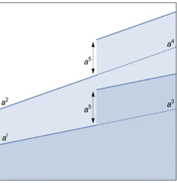
6.1.2. Model 2(three layer with fault). This model is described in[16], where it is labelledtest model 1. The geometric parametersa=₍a a1, 2,a3,a4,a5_{)are defined as infigure8, with the} fault occurring at x=0.55. For simulations, we use the choice of prior

m n

= ´ ´

-= ´ ´

-- -

-N A N A N A

U S U S U

2, 2 0, 2, 2 ,

0.3, 0.3 ,

0 1.4 1.8 1.4

0

( ) ( ) ( )

( ) ( ) ([ ])

whereS Í_[0, 1_]2 _{is the simplexS={(x y, ) ∣0}  _{x 1,x} _{y 1}.}

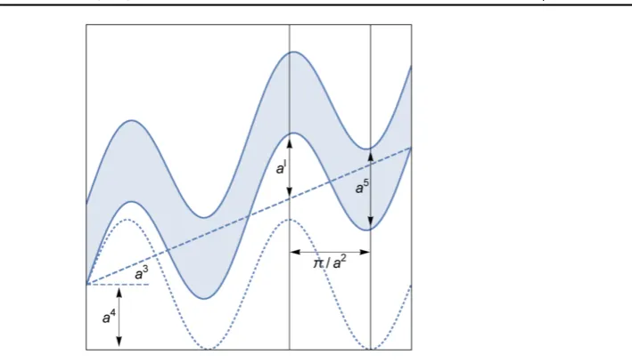
6.1.3. Model 3(channel). This model is described in[16], where it is labelledtest model 2. The geometric parameters a =₍a a1, 2,a3,a4,a5_{) are de}fi_{ned as in} fi_{gure 9. Here} a a1, 2,a3,a4,a5_{represent the channel amplitude, frequency, angle, initial point and width} respectively. For simulations, we use the choice of prior

m

n p p p p

= ´

-= ´ ´ - ´ ´

-

-N A N A

U U U U U

1, 1, ,

0, 1 , 4 4, 4 0, 1 0, 0.4 .

0 1.4 1.8

0

( ) ( )

([ ]) ([ ]) ([ ]) ([ ]) ([ ])

For each model, we fix a true permeability (u†,a†) _{as a draw from the corresponding}

prior distribution, generated on a mesh of 2562points. For the forward model, we take the coefficient map s(·)=exp(·). We observe the pressure on a grid( )xi i25₌1 of 25 uniformly spaced points, via the maps (2.4) withe=0.05. We add i.i.d. Gaussian noise N₍0,g2_{) to} each observation, taking g=0.01. The resulting relative errors on the data can be seen in Figure 9. The definition of the geometric parameters a=₍a a1, 2,a3,a4,a5_{) in} model 3.

Table 1.The relative error on the data, when each measurement is perturbed by an instance ofN₍0, 0.012_{) noise.}

Model number Mean relative error(%) Range of relative errors(%)

1 0.5 0.02–3.5

2 0.9 0.1–4.0

table 1. Small relative errors of this size typically make the posterior distribution hard to sample as they lead to measure concentration phenomena; MAP estimation can thus be particularly important.

6.2. MAP estimation

Based on the theory in section 5, we can calculate MAP estimators by minimising the Onsager–Machlup functional for the posterior distribution. We compute local minimisers of the Onsager–Machlup functional using the following iterative alternating method.

Algorithm 6.1.

(1) Choose an initial state(u0,a0)ÎX´ L.

(2) Update the geometric parameters simultaneously using the Nelder–Mead algorithm.

(3) Update eachfield individually using a line-search in the direction provided by the Gauss– Newton algorithm.

(4) Go to 2.

The Nelder–Mead and Gauss–Newton algorithms are discussed in [30], in sections 9.5 and 10.3 respectively. Since we do not update the fields and geometric parameters simulta-neously, it is possible that this algorithm will get caught in a saddle point: consider for example the function f :´, f x y( , )=xy, at the point(0, 0), being minimised alternately in the coordinate directions. Hence once the algorithm stalls, we propose a large number of random simultaneous updates in an attempt tofind a lower functional value. If this is successful, we return to step (2)of the algorithm. We terminate the algorithm once the difference between successive values ofΦis below TOL=10−5. Calculations are performed on a mesh of 642points in order to avoid an inverse crime.

To ensure that we explore the support of the posterior distribution, we choose a variety of initial states (u0,a0)ÎX´ L for the minimisation such that I u( 0,a0)< ¥ in the con-tinuum setting. To this end, we leta0be a draw from the prior distributionn0, and takeu0to lie in the Cameron–Martin space of m₀. Specifically, if a component of uÎX has prior distribution N m A( , -a), we take the corresponding component of u0 to be a draw from

a

-N m A₍ , d 2_{). Output of the algorithm is shown infigures10–12.}

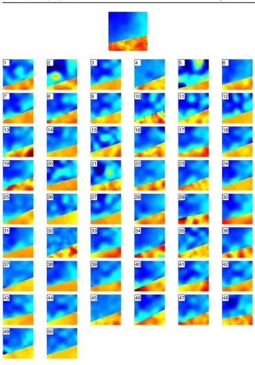
Wefirst comment on the minimisers of the Onsager–Machlup functional for model 1. Generally the geometric parameters are closely recovered regardless of the initialisation state, though there is more variation in thefields. In the simulations where the geometry is inac-curate, for example simulations 7, 17 and 46, thefields can be seen to be compensating by forming a ‘soft’interface where the true interface is.

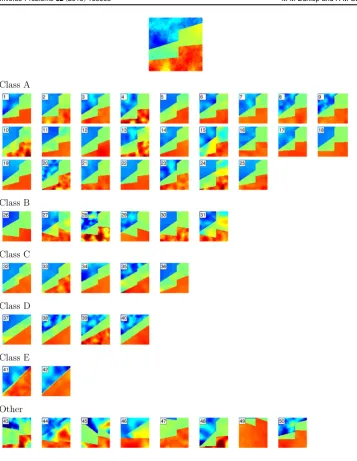
The minimisers associated with model 2 admit much more variation, though it is possible to partition them into smaller subsets of minimisers which share similar characteristics to one another, as mentioned in point (iv) at the beginning of the section. The clustering of the different minimisers is performed by eye, classifying them according to similar geometric parameters. Additionally we have an other class, containing the minimisers which do not appear similar to one another nor appear tofit into any other class. We see later with MCMC simulations that these states do still act as local maximisers of the posterior probability.

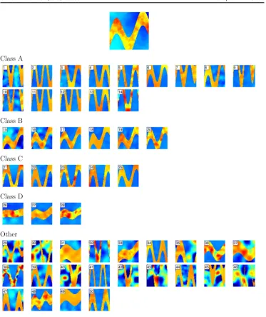
Figure 10.(Model 1)The true log-permeability field(top), and 50 local minimisers arising from minimisation initialised at draws from a smoothed prior distribution. Simulation 12 has the lowest functional value, withI uMAP,a =2847

12 MAP 12

and is echoed in the MCMC simulations later. The other class here is much larger than for model 2, though as with model 2 these states do appear to act as distinct local maximisers of the posterior probability.

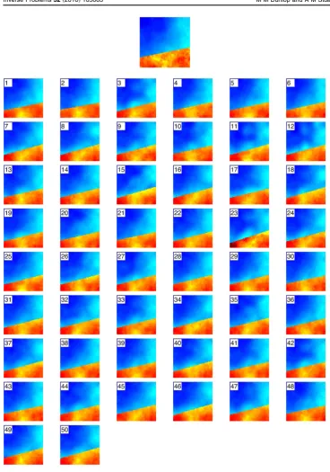
This multi-modality of the posterior distribution is not unexpected. The paper [5] con-siders the history matching problem in reservoir simulation, in which inference is done jointly on both geometric and permeability parameters in the IC fault model. Though the forward Figure 11.(Model 2)The true log-permeability field(top), and 50 local minimisers arising from minimisation initialised at draws from a smoothed prior distribution. Simulation 7 has the lowest functional value, with I uMAP,a =2567

7 MAP

7

( ) . The

map and observation maps are different in our model, we observe the same clustering of nearby local MAP estimators, and increased multi-modality as the dimension of the parameter space increases. In[5]it is observed that the global minimum often does not correspond to the truth, especially in the presence of measurement noise, and so all local minimisers of the Onsager–Machlup functional should be sought before drawing conclusions about the per-meabilities—this appears to be the case in our model as well. We note that MCMC can be Figure 12.(Model 3)The true log-permeability field(top), and 50 local minimisers arising from minimisation initialised at draws from a smoothed prior distribution. Simulation 20 has the lowest functional value, with I u( MAP20 ,aMAP20 )=2117. The