Dynamics of degree two quasiregular mappings of the plane of constant dilatation

(1)

University of Warwick institutional repository: http://go.warwick.ac.uk/wrap

A Thesis Submitted for the Degree of PhD at the University of Warwick

http://go.warwick.ac.uk/wrap/54680

This thesis is made available online and is protected by original copyright.

Please scroll down to view the document itself.

(2)

AUTHOR: Robert Neil Fryer DEGREE: Ph.D.

TITLE: Dynamics of Degree Two Quasiregular Mappings of the Plane of Constant Di-latation

DATE OF DEPOSIT: . . . .

I agree that this thesis shall be available in accordance with the regulations governing the University of Warwick theses.

I agree that the summary of this thesis may be submitted for publication.

I agree that the thesis may be photocopied (single copies for study purposes only).

Theses with no restriction on photocopying will also be made available to the British Library for microlming. The British Library may supply copies to individuals or libraries. subject to a statement from them that the copy is supplied for non-publishing purposes. All copies supplied by the British Library will carry the following statement:

Attention is drawn to the fact that the copyright of this thesis rests with its author. This copy of the thesis has been supplied on the condition that anyone who consults it is understood to recognise that its copyright rests with its author and that no quotation from the thesis and no information derived from it may be published without the author's written consent.

AUTHOR'S SIGNATURE: . . . .

USER'S DECLARATION

(i) I undertake not to quote or make use of any information from this thesis without making acknowledgement to the author.

(ii) I further undertake to allow no-one else to use this thesis while it is in my care.

DATE SIGNATURE ADDRESS

. . . .

. . . . . . . .

. . . .

(3)

Dynamics of Degree Two Quasiregular Mappings of

the Plane of Constant Dilatation

by

Robert Neil Fryer

Thesis

Submitted to the University of Warwick

for the degree of

Doctor of Philosophy

Mathematics

(4)

List of Figures

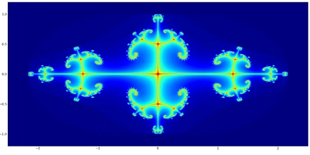
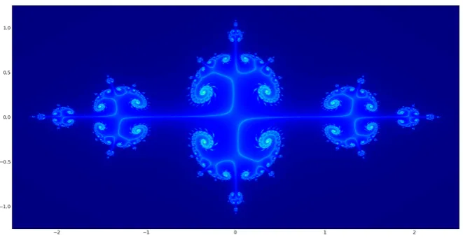
2.1 The black region denotesN(f−1+0.1i). . . 11

2.2 The black region denotesN(fi). . . 11

2.3 The white denotesN(f0.285), the blue regions are points inI(f0.285). . . 12

2.4 The black region denotes the Mandelbrot set, M. . . 12

2.5 How the maps lift to H, with points γ(βi) tending toγ(β). . . 19

3.1 N(fK,θ,c)for K = 1.2, θ= 0.7π and c= 2.297−0.295i. . . 29

3.2 N(fK,θ,c)for K = 0.8, θ= 0 andc=−1.1. . . 29

3.3 N(fK,θ,c)for K = 0.8, θ= 0 andc=−1.1 + 0.003i. . . 30

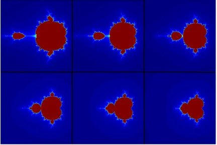
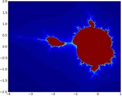
3.4 M_K,₀ for, starting top left and moving clockwise, K = 0.7,0.8,0.9,1.2,1.1 and 1. 31 3.5 M₀_.₇_,π/₁₂ . . . 32

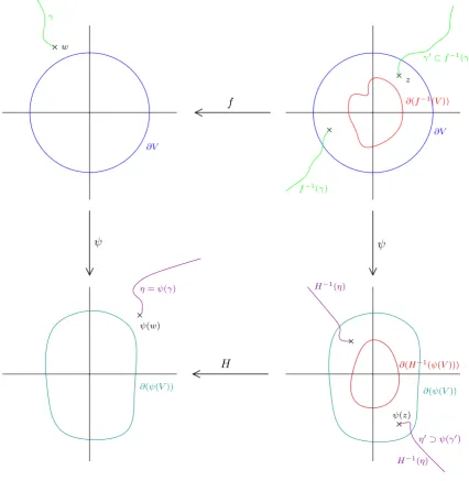
5.1 How ψ extends tof−1(V) . . . 61

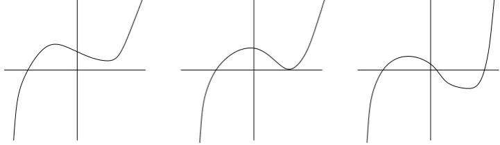
6.1 How the cubicP may vary withK to give, 1, 2 or 3 xed rays. . . 63

6.2 How the cubicP may vary withK to give, 1 or 3 xed rays. . . 64

6.3 Diagram showing the regions F±_θ. . . 67

6.4 Diagram showing howHe is induced from the action ofH on the rayRϕ. . . 68

6.5 Diagram showing the local dynamics ofφi in the two cases. . . 73

6.6 Example of whenHe has two xed points. . . 77

6.7 Example of whenHe has one xed point. . . 79

6.8 Example of whenHe has three xed points. . . 79

6.9 How the xed points of He_K,θ may vary as we vary K for a xed θ6= 0. . . 81

6.10 How the xed points of He_K,θ may vary as we vary θfor a xed K ≤2. . . 84

(8)

6.12 A further example of how the xed points of He_K,θ may vary as we vary θ for a

xedK >2. . . 86

6.13 Diagram showing the local dynamics of one, two and three xed points. . . 89 6.14 Diagram for θ= 0 showing how we obtain a Möbius map with two xed points. . 90

(9)

Acknowledgments

Thanks to my de facto supervisor Alastair Fletcher for introducing me to this subject, explaining many things I should really have known, reading some of my poor attempts at proofs without despairing too much, and generally making writing this thesis a pleasant experience. Thanks also to my supervisor Vladimir Markovic for all his help and understanding and Oleg Kozlovski for agreeing to be my ocial supervisor for the past year. I would also like to thank Mark Pollicott, Saul Schleimer and Sebastian van Strien for their help and advice. Thanks to Adam Epstein and Gwyneth Stallard for agreeing to be my examiners and for their excellent corrections, which have greatly improved this thesis. I am grateful to the EPSRC for funding my PhD.

I must also thank my parents for their support all of my life, my grandma for her al-ternative education when I was o school, my uncle Richard for gently persuading me to study maths at university and my maths teacher Mr Wright for rst introducing me to some of the delights of mathematics!

Writing this thesis would have been much less enjoyable without everyone at the Swim-ming and Water Polo, and Athletics clubs; so thanks to everyone there for all the time I have spent training, competing and socalising. Thanks to my various housemates Azzie, Nick, Tom and Charlie for putting up with me. Also thanks to everyone from N-top for all the fun times and Mike for all the tea breaks! Thanks to Amy, Jonny, Joel, Rob Chapman, Joe, Rob Jolly, Jack, Tristan, Colin, Helen, Matty, Neil, Luke and Mark for trips to various festivals, races and holidays to keep me sane from all the maths. Thanks also to everyone I have shared an oce with, including Tom for all the help with the crosswords and Sarah for all the cake!

(10)

Declarations

I declare that this thesis has not been submitted for a degree at another university.

Chapters 2 and 3 are introductory and survey some material on complex and quasiregular dynamics, based on various sources including [1, 4, 5, 10, 20, 29]. The remaining work is original and includes material from the paper [17] and the preprint [18] coauthored with Alastair Fletcher and presented here in more detail, with some extra diagrams.

(11)

Abstract

Let h:C→Cbe an R-linear map. In this thesis, we explore the dynamics of the quasiregular

mapping h(z)2+c.

It is well-known that a polynomial can be conjugated by a holomorphic mapφtow7→wd

in a neighbourhood of innity. This mapφis called a Böttcher coordinate forf near innity. We

construct a Böttcher type coordinate for compositions ofhand polynomials, a class of mappings

rst studied in [19]. As an application, we prove that if h is ane and c∈_C, then h(z)2+c is

not uniformly quasiregular. Via the Böttcher type coordinate, we are able to obtain results for any degree two mapping of the plane with constant complex dilatation.

(12)

Karma police arrest this man, he talks in maths,

he buzzes like a fridge, he's like a detuned radio.

(13)

Chapter 1

Introduction

The eld of complex dynamics was rst popularised nearly a century ago by Fatou [15, 16] and Julia [27]. Earlier work by Böttcher [8] and others had focused on the linearisability of analytic functions in neighbourhoods of xed or periodic points. In these neighbourhoods the dynamics is well understood and there is some sense of stability. Julia and Fatou were concerned with the iteration of rational functions of the plane. Independently, they studied the boundary of the sets where linearisation was possible; informally this was the set of points where the iterates were badly behaved, these sets are now known as Julia sets. Fatou was concerned with the set of points where the iterates were not a normal family. Julia studied the closure of the set of repelling periodic points. Later it was proved that these two sets were equivalent.

They showed these maps had rich chaotic behaviour on the Julia set. Further Julia knew that quadratic polynomials, when iterated, had Julia sets that were either connected or totally disconnected and that the orbit of the only critical point determined which case occurred. However Julia never studied the parameter that caused this. Research into the area of complex dynamics largely ground to a halt, due to the fact that a complete classication of the stable domains (which became known as the Fatou set) eluded proof. Although notably Baker [34] did much work on the iteration of entire transcendental mappings in this time.

However, interest into complex dynamics was renewed in the 1980s when Sullivan [35], Douady and Hubbard [12], and others introduced powerful new techniques to the subject, in-cluding quasiconformal mappings. Further, computer generated images of Julia sets and the Mandelbrot set created wider interest in the subject outside of the eld itself. They showed the wonderful intricacies at play for functions that could be stated very simply.

(14)

extended to more general functions. In particular we are concerned with quasiregular maps of the plane. Recall that a holomorphic function sends innitesimal circles to innitesimal circles; informally a quasiregular mapping sends innitesimal circles to innitesimal ellipses and the greater the eccentricity of the ellipses, the greater the distortion of the mappings. Quasiregular mappings can be dened in any dimension, see Rickman's monograph [33] for more details.

The rst quasiregular mappings to be iterated were uniformly quasiregular mappings, these are mappings with a uniform bound on the distortion of the iterates, for example holomor-phic functions. These are special cases; in particular, due to Hinkkanen [23], every uniformly quasiregular mapping of the plane is quasiconformally conjugate to a holomorphic function. For more on uniformly quasiregular dynamics see for example [24, 26].

For general quasiregular mappings it is dicult to dene the Fatou set, as we may not have a common bound on the distortion of the iterates and so may not have normality. We do not have an analogue of Montel's Theorem for general quasiregular mappings, which is a key ingredient in proofs of complex dynamics, hence we cannot just adapt existing proofs for their quasiregular analogues. It is however always possible to dene the escaping set I(f) of

a quasiregular mapping f, this is the set of points z such that fn(z) → ∞ as n → ∞. It is

well known that for an analytic function, the boundary of I(f) coincides with the Julia set of

f. Therefore it is natural to consider ∂I(f) as a substitute for the Julia set of quasiregular

mappings. However it is much harder to prove analogous results with the holomorphic case due to the fact we can no longer use any results that use normality. Fletcher and Goodman [19], and Fletcher and Nicks [21] showed that for certain quasiregular mappings we can obtain analogous results for the sets∂I(f)compared to Julia sets of holomorphic functions.

Further, Fletcher and Goodman [19] studied the quasiregular mappings

fK,θ,c(z) :=hK,θ(z)2+c,

where hK,θ is an ane stretch of magnitude K in direction θ and c ∈C. These mappings are

quasiregular analogues of the quadratic polynomialsfc(z) =z2+cthat were studied by Douady and Hubbard. They showed many similar properties to the iteration of quadratic polynomials and they introduced quasiregular versions of the Mandelbrot set, that depend on the parameters

K and θ.

In this thesis we will continue the study of the dynamics of these quasiregular mappings

(15)

the form fK,θ,c, for some K > 1 and θ∈ (−π/2, π/2]. We will construct Böttcher coordinates

that conjugatefK,θ,c to fK,θ,0 :=HK,θ on some neighbourhood of innity. We will see that we have rays that are xed under the mappingsHK,θ. These will play a key role in the dynamics

of HK,θ. In particular we can calculate the complex dilatation of iterates ofHK,θ for points on the xed rays, by seeing they are equal to iterating a Möbius mapping that is dened on each xed ray. We then use these results to show thatHK,θ, and so fK,θ,cby the Böttcher coordinate result, is nowhere uniformly quasiregular. Finally we use more results from the iteration of Möbius maps to obtain certain conditions on maps not being quasiconformally conjugate on any neighbourhood of innity.

1.1 Outline of thesis and key results

In Chapter 2 we survey some complex dynamics and include some results that will be needed later on logarithmic coordinates and hyperbolic Möbius maps of the disk D. Chapter 3 introduces

quasiregular mappings and some of their properties, we then go on to mention some known results including those relevant to the direction we will explore. In Chapter 4 we dene the ane stretch hK,θ and the maps H = HK,θ = (hK,θ)2 and f = fK,θ,c = (hK,θ)2 +c, which will be the main objects that we will study. We show that any degree two quasiregular map of polynomial type of constant complex dilatation is linearly conjugate to this special form.

Proposition 4.1. Let f :C→Cbe quasiregular of degree two and let f have constant complex

dilatation that is not identically0. Thenf is linearly conjugate to a unique mapping of the form fK,θ,c(z) :=hK,θ(z)2+c for someK >1, θ∈(−π/2, π/2]and c∈C.

In Chapter 5 we prove the following theorem, a quasiregular version of Böttcher coordi-nates.

Theorem 5.1. Leth:C→Cbe an ane mapping andc∈C. Then there exists a neighbourhood

U =U(h, c) of innity and a quasiconformal map ψ=ψ(h, c) such that

h(ψ(z))2=ψ(f(z)), (1.1)

for z∈U, where f(z) =h(z)2+c. Further, ψ is asymptotically conformal as |z| → ∞.

A ray is a semi-innite line Rφ={teiφ :t≥0}. In Chapter 6 we consider xed rays of

(16)

Theorem 6.1. Let θ ∈(−π/2, π/2)\ {0}, K > 1 and let H(z) =hK,θ(z)2. Then there exists

Kθ>1 such that:

• for K < Kθ, there is one xed ray that is locally repelling;

• for K = Kθ, there are two xed rays, one of which is locally repelling and one that is

neutral. Further, the neutral xed ray is repelling on one side and attracting on the other;

• for K > Kθ, there are three xed rays, one of which is locally attracting and two that are

locally repelling.

Whenθ= 0the rst and third statements above hold, but when K=Kθ there is just one neutral xed ray which is locally attracting on both sides. When θ=π/2 there is only one xed ray for

all K >1 and it is always locally repelling.

We then go on to study the preimages of their xed rays and basins of attraction. These are the sets Λ⊂Csuch that arg[H_K,θn (z)]→φfor z∈Λ, whereφ is the angle of the attracting

xed ray, Rφ, of HK,θ. In particular we prove the following key result.

Theorem 6.2. If H has one xed ray Rφ then {H−k(Rφ)}∞k=0 is dense in C. If H has two or

three xed rays, then Λ is dense in C.

We use these results to show thatCdecomposes nicely into dierent dynamical sets.

Corollary 6.3. Let K >1, θ∈(−π/2, π/2] and H(z) =hK,θ(z)2. Then C=I(H)∪∂I(H)∪

A(0), where A(0)is the basin of attraction of the xed point 0.

In Chapter 7 we show that our mappingsHK,θ, and sofK,θ,c by the Böttcher coordinate result, are nowhere uniformly quasiregular. We will dene a nowhere uniformly quasiregular mapping later, but informally it is a mappingf that for all pointsz∈_Cand every neighbourhood

U 3z there exists w∈U such thatf is not uniformly quasiregular atw, that is the distortion

of the iterates off is not bounded at w.

Theorem 7.3. Let K > 1 and θ ∈ (−π/2, π/2]. Then the mapping hK,θ(z)2 +c is nowhere uniformly quasiregular.

Finally in Chapter 8 we use a Möbius map, that is derived from the dilatation on xed rays, to give the following conditions on our mapsHK,θ, and againfK,θ,c, not being

quasiconfor-mally conjugate on any neighbourhood of innity. Denote the xed rays ofHK1,θ1 :=H1 byRφi

(17)

xed rayRφi by Ai(z) and the corresponding Möbius transformations of each xed ray Rψj by

Bj(z), where

Ai(z) =

µ+e−iφi_z 1 +e−φiµz,

whereµ=e2iθ1₍_K

1−1)/(K1+ 1)∈Dand

Bj(z) =

ν+e−iφj_z 1 +e−φj_νz,

whereν =e2iθ2₍_K

2−1)/(K2+ 1)∈D. Then we prove the following theorem.

Theorem 8.1. With the notation above, there is no quasiconformal conjugacy between H1 and

H2 in any neighbourhood of innity if any of the following conditions hold:

(i) the mappings H1, H2 have dierent numbers of xed rays;

(ii) H1 and H2 both have one xed ray, Rφ1 and Rψ1 respectively, andTr(A1)

2 ₆_{= Tr(}_B 1)2;

(iii) if H1 and H2 both have two xed rays Rφi and Rψi for i = 1,2, where φ1 > φ2 and

ψ1> ψ2, and Tr(Ai)26= Tr(Bi)2 for some i;

(iv) if H1 and H2 both have three xed rays Rφi and Rψj, i, j ∈ {0,1,2} respectively, where

φ1> φ0 > φ2 andψ1 > ψ0> ψ2, and Tr(Ai)26= Tr(Bi)2 for some i.

Then we reduce the possibility of a quasiconformal equivalence existing on a neighbour-hood of innity, when we x one of K or θto the possible cases given in the following theorem.

Theorem 8.2. • If K >1 is xed and θ1, θ2 ∈(−π/2, π/2) then HK,θ1 and HK,θ2 are not

quasiconformally conjugate on any neighbourhood of innity, except if θ1 =θ2 or possibly

one case whereHK,θ1 and HK,θ2 both have one xed ray and

θ1=φ−tan−1

K

tan(φ−θ2)

,

where φis the xed point of He_K,θ₁ andHe_K,θ₂.

• If θ ∈(−π/2, π/2) is xed and K1 6=K2 >1 then HK1,θ and HK2,θ are not

(18)

Chapter 2

Complex Dynamics

Complex dynamics was originally concerned with the behaviour of rational functions under iteration. Many results have been extended to more general mappings, such as for example to entire functions. We are interested in seeing whether the concepts and ideas of complex analysis can be extended to quasiregular maps. We begin with an overview of some relevant complex dynamics.

2.1 Rational functions

We say f : C → C is a rational function if it can be expressed as f(z) = P(z)/Q(z) where

P, Q:C→Care polynomials. Here C:=C∪ {∞} denotes the Riemann sphere. Recall that a

family of functions is called normal if there is nice behaviour, we dene this more precisely now.

Denition 2.1. A family,F, of meromorphic functions on a domainD ⊂_Cis a normal family

if every sequence {fk} in F contains a subsequence that converges uniformly in the spherical metric, on compact subsets of D, to a meromorphic functionf.

The basic objects studied in the iteration of rational functions, introduced by Fatou [15, 16] and Julia [27], are dened as follows.

Denition 2.2. The Fatou set of the rational function f is dened as:

F(f) :=

n

z∈_C| {fk}_k∈N is normal in some neighbourhood ofz

o

.

The Julia set off is dened as:

J(f) :=nz∈_C| {fk}_k∈_N is not normal in some neighbourhood ofz o

(19)

Also recall Montel's Theorem, which is invaluable in holomorphic dynamics.

Theorem 2.3 (Montel's Theorem, [10] Theorem 3.2). A family of meromorphic functions on

D omitting three xed values is normal.

Let's x some notation. For z∈Clet

O+(z) :={fn(z)|n≥0}

be the forward orbit ofz, let

O−(z) := [

n≥0

f−n(z) = [

n≥0

w∈_C|fn(w) =z

be the backward orbit ofz, and let

O(z) :=O+(z)∪O−(z)

be the orbit ofz. For A ⊂_Cwe letO±(A) =∪_z∈AO±(z)and we say Ais completely invariant

if O(A) =A. Ifξ is an attracting periodic point of periopp, then

Λ(ξ) :=

n

w∈C

_nlim_→∞f

pn₍_w_{) =}_ξo

is the basin of attraction of ξ. The exceptional set E(f) is dened as the set of all points

whose backwards orbit is nite. Given this notation we list some results noted in the review of Bergweiler [5]. This rst theorem summarises some of the results shown by Fatou and Julia.

Theorem 2.4 ([5] Theorem 2.1). Let f be a rational function of degree at least 2. Then:

(i) F(f) is open and J(f) closed.

(ii) F(fn) =F(f) andJ(fn) =J(f) for all n∈_N.

(iii) F(f) and J(f) are completely invariant. (iv) J(f) is perfect.

(v) If X ⊂C is closed and completely invariant and if|X| ≥3, then X ⊃J(f).

(vi) If ξ is an attracting periodic point, then Λ(ξ)⊂F(f) and ∂Λ(ξ) =J(f).

(20)

(viii) |E(f)| ≤2 and E(f)∩J(f) =∅.

(ix) If z∈J(f) then J(f) =O−(z).

Another basic result of the dynamics of rational functions is the following.

Theorem 2.5 ([4] Theorem 4.2.7). The Julia set of a rational function is the closure of the set of repelling periodic points.

2.1.1 Polynomials

A special set of rational functions is the set of polynomials. All polynomials x the point at innity; further innity is always an attracting xed point if we require the degree to be greater than one. We dene the escaping set of a mapping f to be

I(f) :={z∈_C|fn(z)→ ∞asn→ ∞}.

We can also dene the non-escaping set, the set of points that remain bounded under iterations of f, as

N(f) :=C\I(f).

Note that here we use N(f) instead of the usual K(f), so as not to confuse the non-escaping

set with the distortion of f. If f is a polynomial of degree d≥ 2, then we always have ∞ as

an attracting xed point and there always exists some neighbourhood U of innity such that U ⊂I(f). Also whenf is a polynomial we can obtain an estimate on large values ofz.

Lemma 2.6. Letf :C→C be a polynomialf(z) =anzn+an−1zn−1+· · ·+a0 where n ≥ 2,

ai∈Cand an6= 0. Then there exists some R >0 such that if |z|> R then |f(z)| ≥2|z|. Remark 2.7. Notice that this lemma implies that if |z| ≥ R then z∈I(f). In fact we can do

even better and note; if |fm(z)| ≥R for somem∈_N, then z∈I(f).

Proof. We can chooseR large enough so that if|z| ≥R then

|an||z|n

2 ≥2|z|,

and

|an||z|n

2 ≥ |an−1||z|

n−1₊_{· · ·}₊_|_a

(21)

Then if|z| ≥R,

|f(z)| ≥ |an||z|n−(|an−1||z|n−1+· · ·+|a1||z|+|a0|)≥ 1 2|an||z|

n_≥₂_|_z_|_.

The motivation behind introducing the escaping set is the following result linking it to Julia sets.

Proposition 2.8. If f is a polynomial then J(f) =∂I(f).

Remark 2.9. The proof of this is immediate from part (vi) of Theorem 2.4, but we include a proof to show the methods at play.

Proof. First we showI(f)is open. Ifz∈I(f)then|fm(z)|> Rfor somem∈_N, for anyR >0.

By continuity there exists some ε >0 such that|fm(w)|> R for allw∈Bε(z). By Lemma 2.6 and the remark afterwards,w∈I(f) showingI(f)is open.

Pick z ∈ ∂I(f). Then every neighbourhood U 3 z contains points w ∈ U such that fn(w) → ∞ as n → ∞, but fn(z) remains bounded. Hence no subsequence of {fn(z)} is

uniformly convergent onU; hence{fn}is not normal at z, soz∈J(f) and

∂I(f)⊂J(f). (2.1)

Now suppose z /∈ ∂I(f). Then either z ∈I(f)\∂I(f) or z ∈ _C\(I(f)∪∂I(f)). If z ∈ I(f)

then, as it is not on the boundary, there exists a neighbourhoodV 3zsuch thatV ⊂I(f), then

fn(w)→ ∞ asn→ ∞for all w ∈V, hence fn converges uniformly to innity on V and {fn}

is normal at z. If z ∈ _C\(I(f)∪∂I(f)) then there exists a neighbourhood V 3 z and some C >0 such that|fn(w)|< C for allw∈V. Applying Theorem 2.3 we see that {fn} is normal

at z. Hencez /∈J(f) and (∂I(f))c= (J(f))c, using this and (2.1) we seeJ(f) =∂I(f).

2.1.2 Quadratic polynomials

We will be investigating a quasiregular version of quadratic polynomials and so mention some more results focusing on this.

Proposition 2.10. Any quadratic polynomial of the formP(z) =αz2+βz+γ, whereα, β, γ∈_C

(22)

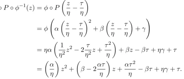
Proof. Letφ(z) :=ηz+τ, where η, τ ∈_Candη 6= 0; then φ−1(z) =z/η−τ /η. Let us consider φ◦P◦φ−1(z) =φ◦P

z η − τ η

=φ α

z η − τ η 2 +β z η − τ η +γ ! =ηα 1

η2z 2₋₂ τ

η2z+

τ2

η

+βz−βτ +ηγ+τ

=

α η

z2+

β−2ατ

η

z+ατ 2

η −βτ+ηγ+τ. (2.2)

We are trying to show fc=φ◦P◦φ−1 for somec. Hence by (2.2) we requireα =η and

β = 2ατ /η, this impliesβ = 2τ. Hencec= (3β2_{+ 2}_β₎_/_{4 +}_αγ_.

The advantage of conjugating every quadratic polynomial to somefcis that 0 is now the only branch point. Recall the denition of the set of branch points of a mapping.

Denition 2.11. Let f : C → C be a continuous mapping. Then B(f) := {z ∈ C |f is not

locally injective atz}, denotes the branch set off.

LetJc:=J(fc), then we have the following Theorem proved in [10].

Theorem 2.12 ([10] VIII. Theorem 1.1). If f_cn(0) → ∞ as n → ∞ then the Julia set Jc is totally disconnected. Otherwise f_cn(0)is bounded and Jc is connected.

We now illustrate these concepts by considering some examples of N(fc) for dierent values ofc∈_C, gures are shown on the next two pages.

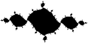
Figure 2.1 depictsN(f−1+0.1i); in this case0∈/I(f−1+0.1i)and so the Julia set,J−1+0.1i=

∂I(f−1+0.1i) = ∂N(f−1+0.1i), is connected. Also notice that the interior of N(f−1+0.1i) is non-empty.

[image:22.595.157.453.104.231.2]

Figure 2.2 depictsN(fi); in this case0∈/ I(fi) and so the Julia setJi is connected. Also notice that the interior ofN(fi)is empty, so N(fi) =Ji.

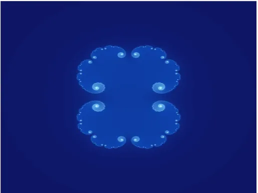
Figure 2.3 depicts N(f0.285); in this case 0∈/ I(f0.285) and so the Julia set J0.285 is not

connected and is again equal to N(f0.285), in fact it is totally disconnected. The reason some

regions look connected is due to the fact that nearby points escape very slowly and so more iterations would be needed for a more dened picture. Also by Theorem 2.4 we know that

J0.285 is perfect, this means given z∈J0.285 every neighbourhoodU 3z has the property that

(23)

[image:23.595.223.373.150.224.2]

Figure 2.1: The black region denotesN(f−1+0.1i).

Figure 2.2: The black region denotes N(fi).

The pointsc∈_CwhereJcis connected is known as the Mandelbrot set, denoted by M. In our examples c=−1 + 0.1iand c=iare points of Mbut c= 0.285is not contained inM.

(24)

[image:24.595.169.427.71.264.2]

Figure 2.3: The white denotes N(f0.285), the blue regions are points inI(f0.285).

Denition 2.13. The Mandelbrot set is dened as

M:={c∈C|fcn(0)is bounded}.

Figure 2.4: The black region denotes the Mandelbrot set,M.

Many results have been proved about the Mandelbrot set, we will mention some of these briey.

[image:24.595.142.454.396.626.2]

(25)

D2 := {|c|<2} ⊂ C, which meets the real line in the interval [−2,1/4]. Further c∈ M if and

only if f_cn(0)≤2 for all n∈N.

By denition if c∈ M thenJc is connected however, as can be seen in Figures 2.1 and 2.2, we have cases where N(f) has non-empty and empty interior respectively. If c is in the

interior ofMthenN(fc)has non-empty interior, however this may still be the case forc∈∂M. Points c ∈ ∂M where N(fc) has empty interior are called Misiurewicz points. There is much literature about iterations of quadratic polynomials and the Mandelbrot set, see for instance [4, 10, 11, 14].

2.2 Logarithmic coordinates

To prove Theorem 5.1, we will need to use the logarithmic transform which we briey outline here.

Let f be a function dened in a neighbourhood U = {|z| > R} of innity and which

grows like a polynomial. That is, there exist constantsA, B, n such that

A≤ |f(z)| |z|n ≤B. Thenf lifts to a function

e

f(X) = logf(eX)

for ReX >logR.

Denition 2.15. The function feis called the logarithmic transform of f, and is unique up to

addition of an integer multiple of2πi.

Lemma 2.16. Supposef, g are two functions whose logarithmic transforms exist. Thenf]◦g=

e

f◦_eg in a suitable neighbourhood of innity.

Proof. We know that f is dened on a neighbourhood of innity Ue. Choose R > 0 large

(26)

neighbourhood of innity g(U). We have,

]

f ◦g(X) = log[f(g(expX))]

= log[fexp(log[(g(expX))])] = log[f(exp[_eg(X)])]

=fe◦_eg(X).

Lemma 2.17. Let g(z) = z2 +c. Then g_e(X) = 2X+ρ(X), where ρ(X) = O(e−2 Re(X)) as Re(X)→+∞.

Proof. We have

e

g(X) = log(e2X +c)

= log(e2X(1 +ce−2X)) = 2X+ log(1 +ce−2X),

which proves the lemma.

2.3 Böttcher coordinates

Böttcher showed the following theorem, which we will prove a quasiregular version of in the next chapter.

Theorem 2.18 ([8]). Letf be holomorphic in a neighbourhoodU of innity, and let innity be

a superattracting xed point of f, that is, there exists n≥2 such that

f(z) =anzn(1 +o(1)),

for z∈U, wherean∈C\ {0}. Then there exists a holomorphic change of coordinate w=ψ(z),

with ψ(∞) =∞, which conjugates f tow7→ wn in some neighbourhood of innity. Further, ψ

is unique up to multiplication by an (n−1)-th root of unity.

The map ψ is called a Böttcher coordinate for f near innity. In Chapter 5 we will nd

(27)

of degree n≥ 2, and h is an ane mapping of the plane to itself. As we will follow a similar

method later, we now prove this following the proof of Milnor ([29] Theorem 6.7).

Proof. Suppose our map has the Laurent series expansion

f(z) =anzn+an−1zn−1+· · ·+a0+a−1z−1+· · ·

where n ≥ 2, which is convergent for |z| > r. First notice that the linearly conjugate map z7→αf(z/α),whereαn−1 =an, has leading coecient 1. So we may assume an= 1. Hence

f(z) =zn(1 +o(1)),

for large |z|. Now we utilise logarithmic coordinates, introduced in the previous section. If we

choose the correct lift we obtain

e

f(X) =nX +O(e−Re(X)), (2.3)

for large enough Re(X). This implies

|fe(X)−nX|<1, (2.4)

for large enough Re(X). Choose σ > 1 large enough so that (2.4) is satised for all X in

the half plane Hσ dened as the points X ∈ C such that Re(X) > σ. By construction fe

maps this half plane into itself. Also as fe(X+ 2πi)−fe(X) is a multiple of 2πi this implies

e

f(X+ 2πi)−fe(X) = 2πinby (2.3) and becausefe(X+ 2πi)−fe(X)andn(X+ 2πi)−nX dier

by at most 2 by (2.4).

SupposeX0 7→X1 7→X2· · · is an orbit underfein_H_σ, then we know|X_k₊₁−nX_k|<1.

SettingWk:=Xk/nk we see

|Wk+1−Wk|<1/nk+1.

Hence the sequence of holomorphic functionsWk =Wk(X0) converges uniformly and

geometri-cally ask→ ∞ to a holomorphic limit

Ψ(X0) = lim

(28)

This mapping satises the identity

Ψ(fe(X)) =nΨ(X).

Also Ψ(X+ 2πi) = Ψ(X) + 2πi, so the mapping ψ(z) =eΨ(log(z)) is well dened near innity

and satises

ψ(f(z)) =ψ(z)n,

as required.

All that is left is to prove uniqueness. It is enough to study mappings ζ 7→ η(ζ) near

innity that satisfyη(ζn) =η(ζ)n. Setting

η(ζ) =c1ζ+c0+c−1ζ−1+· · ·,

this implies

c1ζn+c0+c−1ζ−n+· · ·= (c1ζ+c0+c−1ζ−1· · ·)n=cn1ζn+ncn

−1 1 c0ζ

n−1₊_{· · ·}_.

This implies c1 = cn1. Since c1 6= 0, we have that c1 must be an (n−1)-th root of unity.

Comparing the remaining coecients we see ci= 0 for i6= 1.

Remark 2.19. In particular, iff is a quadratic polynomial then by Proposition 2.10 it is linearly

conjugate to fc(z) = z2+c for some c ∈ C. Then each fc is conformally conjugate to z2 by Theorem 2.18 on some neighbourhood of innity.

2.4 Möbius maps and Blaschke products

To prove theorems in Chapters 7 and 8 we will need some results on hyperbolic Möbius maps of

D. We briey recall some standard denitions and results from hyperbolic geometry; for more

background and detail see [1].

Denition 2.20. Let A:D→ D be a Möbius map, where A(z) = (az+b)/(cz+d) for some

a, b, c, d∈_Rand letλ= 1/√ad−bc. Then

b

A:= λaz+λb

λcz+λd =

b

az+bb b

cz+db

(29)

is the normalised form and

TrA=ba+d.b

Denition 2.21. A Möbius mapA:D→Dis called hyperbolic if Tr(A)2>4and parabolic if

Tr(A)2 = 4.

When A is hyperbolic more is known. There exists a unique geodesic that is preserved

set wise under A and we denote this by Ax(A). Further ifA is a hyperbolic Möbius map of D

then there exist α, β∈∂Dsuch that An(z)→α andA−n(z)→β asn→ ∞ for allz∈D. Also

Ax(A)is the geodesic joiningα andβ. IfAis parabolic then there exists one xed point α∈D

and An(z)→ α asn→ ∞ for all z ∈_D. We will require the following lemma which gives the

standard form for a hyperbolic Möbius map of the upper half plane H.

Lemma 2.22. Let A :D→ D be a hyperbolic Möbius map. Then A is conjugate to a Möbius

map Ae:_H→_Hgiven by

e

A(z) =kz

where

k= (T−2−(T2−4T)12)/2<1, (2.5)

and T := Tr2(A).

Proof. We know thatTr2A >4and so by standard hyperbolic geometry we can lift to the upper

half plane to obtainA:H→H. We see Ahas the same trace as A and is of hyperbolic type so

must be conjugate toAe(z) =kz for some k >0. Conjugation preserves trace hence

k+ 1/k+ 2 = Tr2(Ae) = Tr2(A) =T.

Solving this for k and taking the negative square root gives equation (2.5) and k <1. Taking

the positive square root would give the reciprocal.

The following theorem on sequences of hyperbolic Möbius transformations is a combina-tion of results from [22] and [28].

Theorem 2.23 ([22, 28]). LetA, Aj be hyperbolic Möbius maps ofDsuch thatAn(z)→α∈∂D

(30)

hyperbolic Möbius maps of D dened by

tn(z) =A1◦A2◦. . .◦An(z),

sn(z) =An◦An−1◦. . .◦A1(z).

Then both tn(z)→α and sn(z)→α as n→ ∞ for all z∈D.

We use this result to prove the following theorem, which is a new result.

Theorem 2.24. Let A, Aj :D → D be hyperbolic Möbius maps such that An(z) → α ∈∂D as

n→ ∞ and Aj →A locally uniformly as j→ ∞. Let

tn(z) =A1◦A2◦. . .◦An(z).

Then

dh(0, tn(z)) = log

"

1

Qn

j=1kj

#

+O(1),

for large n, where dh denotes the hyperbolic metric on D, kj < 1 for all j and kj → k, where

kj, k are the quantities dened in Lemma 2.22.

Remark 2.25. In particular, if Aj =A for every j∈N, then

dh(0, An(z)) = log [1/kn] +O(1)as n→ ∞.

Proof. First if An(z) → α for z∈ Dthen tn(z) → α by Theorem 2.23. Now let B =A−1 and

Bj =A−j1. Then ifα, β∈∂Dare the attracting and repelling xed points ofArespectively, then

β is the attracting xed point andα is the repelling xed point of B. Similarly if αj, βj ∈∂D

are the attracting and repelling xed points of Aj respectively, then βj is the attracting xed point and αj is the repelling xed point of Bj. Further, we have Bj → B and so αj → α and

βj →β asj→ ∞.

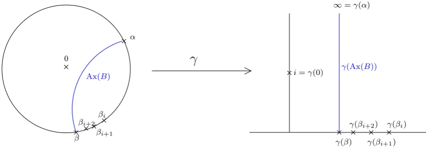
We writeBe for the lift ofB to Hvia γ:D→Hso that Be =γ◦B◦γ−1. We chooseγ so

thatγ(α) =∞ and γ(0) =i. This then means that γ(β) =X ∈_Rand γ(βj) =Xj ∈R, where

Xj →X asj→ ∞.

We can also conjugate by the mapsΦ,Φi :H→HwhereΦ(z) =z−XandΦi(z) =z−Xi. This means that

e

(31)

whereBb(z) = kz and Bb_j(z) = k_jz. The factors k and k_j are determined as in Lemma 2.22 so

thatk, kj <1 and kj →k asj→ ∞.

γ(Ax(B))

γ(β)

γ(βi+2)

γ(βi+1)

γ(βi)

i=γ(0)

∞=γ(α)

β βi+2

βi+1

βi

α

Ax(B)

[image:31.595.84.508.118.275.2]

0

_γ

Figure 2.5: How the maps lift toH, with points γ(βi) tending toγ(β). Let

sn:=t−n1=Bn◦. . .◦B1.

Writing ρ_H for the hyperbolic metric onH, by conformal invariance we have

dh(0, tn(z)) =ρH(i, γ(tn(z))) =ρ_H(i,ten(γ(z))

=ρ_H(s_en(i), γ(z)).

We can rewriteesn(i) as

e

sn(i) = Φ−n1◦Bb_n◦Φ_n◦Φ−_n₋1₁◦Bb_n−1◦Φn−1◦. . .◦Φ1−1◦Bb₁◦Φ₁(i).

It is not hard to see that

e

sn(i) = n

X

j=1



(Xj−1−Xj)





n

Y

i=j

ki



 

+Xn+i n

Y

i=1

ki,

where we use the conventionX0 = 0. Writing

Pn= n

Y

i=1

ki, Rn= n

X

j=1



(Xj−1−Xj)





n

Y

i=j

ki



 



(32)

Rn→0 asn→ ∞. By the formula for the hyperbolic metric inH[1, see 3.4],

ρ_H(s_en(i), γ(z)) = cosh−1

(Rn+Xn−x)2+ (Pn−y)2

2Pny

= cosh−1

Pn

2y + R2

n+Xn2+x2−2xRn−2xXn+ 2XnRn−y

2Pn

. (2.6)

SinceRn→0,Xn→X andx, y are xed,

(R2_n+X_n2+x2−2xRn−2xXn+ 2XnRn−y)−→(X2+x2−2xX−y), (2.7)

asn→ ∞. This expression is bounded. We also have

Pn

2y →0asn→ ∞. (2.8)

Hence, from (2.6),(2.7), (2.8) and using the identitycosh−1(z) = log(z+√z2_{+ 1)}, we can write

ρ_H(_esn(i), γ(z)) = cosh−1

O 1 Pn = log O 1 Pn (2.9) = log 1 Pn

+O(1), (2.10)

which proves the lemma.

We will need to use the following result on Blaschke products, see for example [4, 10]. A Blaschke productB is given by

B(z) :=ζ

n

Y

i=1

z−ai

1−aiz

mi

,

whereζ ∈∂Dand |ai|<1.

We are only concerned with Blaschke products of degree two and in this case we have the following standard result.

Proposition 2.26. LetB be a Blaschke product of degree2. Then the Julia setJ(B)is contained

in S1 and we have the following cases:

• If B has one xed point in S1, one xed point in D and one xed point in C\D, then

(33)

• IfB has one xed point in S1 of multiplicity three, and no other xed points, thenJ(B) =

S1.

• If B has one repelling and one neutral xed point in S1, then J(B) is a Cantor subset of

S1.

• If B has three xed points in S1, then J(B) is a Cantor subset of S1.

This proposition is shown in [10, p58]. However, let's discuss the cases separately. Up to multiplicity B must have three xed points. Ifz0 is a xed point then 1/z0 must be a xed

point also, so there must always be at least one xed point on S1.

Suppose z0 ∈ D is an attracting xed point then the Denjoy-Wol Theorem [10, IV

Theorem 3.1] tells us Bn(z) → z0 for all z ∈ D and also that the xed point on S1 must be

repelling. Using the inversiong(z) = 1/zwe see that1/z0 is an attracting xed point also, such

that Bn(z) → 1/z0 for all z ∈C\D. As J(B) must be the boundary of the attracting basins

of the xed points, this impliesJ(B) =S1. Similarly ifz0 ∈S1 is a xed point of multiplicity

three, then by the Denjoy-Wol TheoremBn(z)→z0 forz∈Dand using the inversiong again

we haveBn(z)→z0 for z∈C\D, henceJ(B) =S1.

If there are three distinct xed points on S1, then the Denjoy-Wol Theorem tells us

that precisely one of them must be attracting and the other two are repelling. J 6=S1 as the

attracting xed point is not in J(B) and so J(B) is a Cantor set in S1. If there is xed point

of multiplicity two, then it must have one attracting direction of points on S1 and J(B) is a

(34)

Chapter 3

Quasiregular maps and dynamics

3.1 Quasiregular maps

A comprehensive study into quasiregular mappings is given by Rickman in his monograph [33], for our purposes the following is more than sucient. Let d >1 and letD ⊂_Rd_{be a domain.} Denition 3.1. Let ACL(D) be the set of all continuous maps f = (f1, . . . , fd) : D → Rd

which are absolutely continuous on almost all lines parallel to the coordinate axes. For a map

f ∈ACL(D) the partial derivatives ∂kfj exist almost everywhere. For p ≥1 we let ACLp(D) denote the set of allf ∈ACL(D) for which all partial derivatives are locallyLp-integrable.

If f : D →Rd is a continuous map, then f ∈ ACLp(D) if and only if f belongs to the

Sobolev spaceW_p,loc1 (D).

Denition 3.2.

W_p,loc1 ={f :D →_Rd| each∂kfj exists and is locally inLp}. Denote the Euclidean norm ofx∈_Rn _by _|_x_|_.

Denition 3.3. A map f ∈ACLd(D) is called quasiregular if there exists a constant KO ≥1 such that

|Df(x)|d≤KOJf(x) a.e.; (3.1)

whereDf(x) denotes the derivative,

|Df(x)|:= sup

|h|=1

(35)

denotes its norm, andJf(x) denotes the Jacobian determinant. Let

`(Df(x)) := inf

|h|=1

|Df(x)(h)|.

The condition that (3.1) holds for someKO≥1is equivalent to the condition that

Jf(x)≤KI`(Df(x)) a.e., (3.2)

for some KI ≥1. The smallest constants KO = KO(f) and KI = KI(f) for which (3.1) and (3.2) hold are called the outer and inner dilation of f. Further K := max{KI(f), KO(f)} is called the dilation off. We say thatf is K-quasiregular ifK(f)≤K.

Note that an injective K-quasiregular map isK-quasiconformal. Further it is clear from

the equations (3.1) and (3.2) that the composition of two, and so inductively a nite number, of quasiregular maps is itself quasiregular.

Lemma 3.4. Iff andgare quasiregular thenf◦gis quasiregular, assuming that the composition

is well dened. Further;

K(f ◦g)≤K(f)K(g).

We denote the one point compactication ofRdbyRd:=Rd∪ {∞}in the usual way (see

for instance [29]). We sayp∈_Rd_{is a pole of a quasiregular mapping}_f _:

Rd→Rdif f(zn)→ ∞ asn→ ∞ for every sequence of points zn that tend top and we writef(p) =∞.

Many properties of holomorphic maps hold for quasiregular maps as well. For example, non-constant quasiregular maps are open and discrete (Chapter I, Theorem 4.1 [33]). Also a modied version of Picard's Theorem is true, shown by Rickman.

Theorem 3.5 ([32] Theorem 1.1). Let d ∈ _N, d ≥ 2, and K ≥ 1. There exists a constant

q =q(d, K) with the following property: if a1, . . . , aq ∈ Rd are distinct points and if f :Rd → Rd\ {a1, . . . , aq} is K-quasiregular, then f is constant.

Equivalently the theorem tells us that a non-constant K-quasiregular mapf :Rd →Rd

omits at most q values. Note that Picard's theorem is a special case of this where q(2,1) = 2.

Also we have an analogue of Montel's Theorem, shown by Miniowitz.

Theorem 3.6 ([30] Theorem 4). Let d≥2 and K ≥1. Let a1, . . . , aq ∈Rd be distinct points,

where q = (d, K) is as in Theorem 3.5. Let Ω ⊂ _Rd _{be a domain. Then the family of all}

(36)

Equivalently this tells us, if a1, . . . , aq ∈ Rd are distinct, then the family of all K

-quasiregular mapsf :Rd→Rd\ {a1, . . . , aq}is normal.

3.1.1 Quasiregular maps of the plane

We will be concerned with quasiregular maps of C, that is we have d= 2, where a lot more is

known. We identify R2 with C and consider quasiregular maps f :D → C, where D ⊂ C is a

domain. For a detailed study see, for instance, [2] or [31]. We have

|Df(z)|=|fz(z)|+|fz(z)|,

`(Df(z)) =|fz(z)| − |fz(z)|, and

Jf(z) =|fz(z)|2− |fz(z)|2

whenever the partial derivatives off exist. It follows that

K(f) =KO(f) =KI(f) =

1 +k

1−k

where

k:= ess sup

z∈D

fz(z)

.

Note that the 1-quasiregular maps are precisely the holomorphic, or meromorphic, func-tions. We also have the following standard denition as with quasiconformal maps, see for example [20].

Denition 3.7. If f : C → C is dierentiable at z then the complex dilatation of f at z is

dened as,

µf(z) =

fz

.

The distortion at zis dened as,

K(f)(z) = 1 +|µf(z)| 1− |µf(z)|

.

We will also require the following useful result about composed mappings.

(37)

and µg. Then

µg◦f =

µf +rf(µg◦f)

1 +rfµf(µg◦f)

,

where rf =fz/fz.

We now state more some results given in the survey [5].

Theorem 3.9 ([5] Theorem 3.3). Let µ:C→C be a measurable function withk:=||µ||∞<1.

Then there exists a K-quasiconformal homeomorphism f :C → C with K := (1 +k)/(1−k)

such that

fz(z)

=µ(z) a.e. (3.3)

The map f may be chosen to x 0,1 and ∞; with this normalisation it is unique.

Equation (3.3) is called the Beltrami equation. A consequence of this theorem is the following.

Theorem 3.10 ([5] Theorem 3.4). Let U, V ⊂_C be simply connected domains with U, V 6=C.

Let µ:U → C be measurable with k := ||µ||∞ <1 and put K := (1 +k)/(1−k). Then there

exists a K-quasiconformal homeomorphism f :U →V such that fz(z)/fz(z) =µ(z) a.e. Notice that the caseµ(z)≡0is the Riemann mapping theorem. Therefore Theorems 3.9

and 3.10 are also called the measurable Riemann mapping theorem. In the plane, every quasireg-ular mapping has a useful decomposition which we will be using extensively.

Theorem 3.11 (The Stoilow factorisation, see for example [26] p.254). Let f : C → C be a

quasiregular mapping. Then there exists an analytic function g and a quasiconformal mapping h such that f =g◦h.

A direct consequence of this and Montel's Theorem is that q(2, K) = 2. The Stoilow

factorisation tells us what the branch set of quasiregular maps of the plane can be. Recall the denition of the set of branch points B(f) from Denition 2.11. A quasiconformal map is a

homeomorphism by denition, so has no branch points. A polynomial must have nitely many branch points, as must a mapping of polynomial type which we dene precisely now.

Denition 3.12. A mapping f :Rn → Rn is said to be of polynomial type if |f(x)| → ∞as

|x| → ∞.

Using this we have the following corollary of the Stoilow factorisation.

Corollary 3.13. Let f :C→C be quasiregular. Then B(f) is a discrete set of points. If f is

(38)

3.2 Quasiregular dynamics

3.2.1 Uniformly quasiregular dynamics

We call a quasiregular mapping f : D → C uniformly quasiregular if there exists K ≥ 1 such

thatKfn(z)≤K for all n∈_Nand for allz∈ D.

Iff is uniformly quasiregular then direct analogues of Fatou and Julia sets can be dened.

However for non-uniformly quasiregular functions,f :C→C, we have no common bound on the

distortion of the family of functions {fk}k∈N, so cannot dene the Fatou set (and so the Julia

set also) easily. It is however still possible to dene the escaping set I(f). By Proposition 2.8

we know J(f) = ∂I(f) when f is a polynomial. In fact this is still true when f is just a

transcendental entire function, shown by Eremenko [13]. It is therefore natural to consider

∂I(f) for quasiregular mappings and see to what extent it can be considered an analogue of

J(f). We will be considering quasiregular mappings of polynomial type, so that innity is an

attracting xed point. We also have the denition of the degree of a quasiregular mapping, which as expected is dened as the maximal cardinality of the preimage of a point of C.

Denition 3.14. The degree of a quasiregular mappingf :C→Cis given by

deg(f) = sup

z∈C

|{f−1(z)}|.

We have the following results on quasiregular mappings of polynomial type from the paper by Fletcher and Nicks [21].

Theorem 3.15 ([21] Theorem 1.1). Letn≥2andf :Rn→RnbeK-quasiregular of polynomial

type. If the degree off is greater thanKI, thenI(f)is a non-empty open set and∂I(f)is perfect.

Notice how these properties are the same as for a polynomial f. Further, compare the

following theorem to the earlier Theorem 2.4 for rational functions to see the similar properties.

Theorem 3.16 ([21] Theorem 1.2). Letf :Rn→Rn be K-quasiregular of polynomial type and

suppose that the degree of f is greater than KI. Then:

(i) for any k≥2 we haveI(fk) =I(f),

(ii) the family of iterates {fk|k∈N} is equicontinuous on I(f) and not equicontinuous

(39)

(iii) ∂I(f) is innite,

(iv) I(f), ∂I(f) and Rn\I(f) are completely invariant,

(v) I(f) is connected.

To see that the condition that the degree of f is greater than KI is necessary, consider the following example.

Example 3.17 ([19] Example 4.1). Consider the winding map f : (r, θ) 7→ (r,2θ) in polar

coordinates. This map decomposes asf =g◦h, whereg(z) =z2 andh(r, θ) = (r12, θ). We have

the following equalities regarding partial derivatives of h,

hz =

1

2(hx−ihy) (3.4)

hz =

1

2(hx+ihy) (3.5)

rhr=xhx+yhy (3.6)

hθ =xhy−yhx. (3.7)

Combining (3.6) and (3.7) we obtain,

hy =

yrhr+xhθ

x2₊_y2 (3.8)

and

hx=

−xrhr+yhθ

x2₊_y2 (3.9)

Using (3.4),(3.5),(3.8) and (3.9) we can obtain an expression for the complex dilatation of h.

µh=

hz

= hx−ihy

hx+ihy

= yhθ−xrhr−iyrhr+ixhθ

yhθ−xrhr+iyrhr+ixhθ

. (3.10)

Grouping partial derivatives and multiplying the numerator and denominator of (3.10) by -1 we see,

µh=

(x+iy)[rhr+ihθ]

(x−iy)[rhr−ihθ]

. (3.11)

Recalling z= x+iy=reiθ, z= x−iy= re−iθ and dividing through by r we are left with the

expression,

µh=e2iθ

hr+ i_rhθ

hr− i_rhθ

. (3.12)

hr=

eiθ

2r12

, hθ=ir

(40)

Hence, by (3.12), the complex dilatation is

µh =

−e2iθ

3 .

So ||µh|| = 1/3 and the distortion of f is 2 and the degree is 2. However I(f) is empty since

|f(z)|=|z|for all z∈_C.

Whenf is uniformly quasiregular we have a bound on the distortion of the iterates. We

can dene the Julia set and have the following result, which is analogous to the case wheref is

a rational function.

Theorem 3.18 ([21] Theorem 1.3). Let n≥2 and f :Rn→Rn be a uniformly K-quasiregular

mapping which is not injective. Then ∂I(f) =J(f) and is an innite, perfect set.

See Hinkkanen, Martin and Mayer [25] for more examples of uniformly quasiregular dynamics.

3.2.2 Quasiregular dynamics in the plane

When we are in the complex plane things are much simpler. We have the very useful Stoilow decomposition of quasiregular functions and also the following theorem due to Hinkkanen.

Theorem 3.19 ([23] Theorem 1). Every uniformly quasiregular map f :C→C is

quasiconfor-mally conjugate to a holomorphic map.

So if we are studying quasiregular dynamics of the plane, then if the map is uniformly quasiregular we can apply results from analytic functions. Hence our study is only of independent interest if we consider non-uniformly quasiregular maps of the plane.

We will see in the next section that there is a quasiregular analogue of quadratic polyno-mials, it is these mappings that we will be studying. Informally they consist of an ane stretch of magnitude K in direction θ, given by hK,θ, then composition with a quadratic polynomial.

We will see in Proposition 4.1 that this composition is linearly conjugate to a special form

fK,θ,c:= (hK,θ)2+c, (3.13)

for K >1, θ∈(−π/2, π/2]and c∈C. The following results are due to Fletcher and Goodman.

(41)

Theorem 3.21 ([19] Theorem 4.5). Let f = fK,θ,c be dened as in (3.13). Then for any

k > 2, I(fk) = I(f). The family of iterates {fk | k ∈ N} is equicontinuous on I(f) and not

equicontinuous at any point of ∂I(f). The set ∂I(f) is innite. The sets I(f), ∂I(f) and I(f)c

are all completely invariant. The escaping set is a connected neighbourhood of innity.

Recall that the non-escaping setN(fK,θ,c) =I(fK,θ,c)c,N(fK,θ,c)is completely invariant by Theorem 3.21. This set N(fK,θ,c) is the analogue of the lled in Julia set for a polynomial. Fletcher and Goodman showed they share similar properties.

Theorem 3.22 ([19] Theorem 5.2). N(fK,θ,c)is connected if and only ifI(fK,θ,c)∩B(fK,θ,c) =∅.

[image:41.595.132.465.286.438.2]

We now consider some examples to visualise these concepts.

Figure 3.1: N(fK,θ,c)for K = 1.2, θ= 0.7π andc= 2.297−0.295i.

[image:41.595.141.458.516.675.2]

(42)

[image:42.595.133.464.69.243.2]

Figure 3.3: N(fK,θ,c) forK = 0.8, θ= 0 and c=−1.1 + 0.003i.

Figure 3.1 showsN(f1.2,0.7,2.297−0.295i); it has non-empty interior and∂I(f1.2,0.7,2.297−0.295i) is connected. Figure 3.2 shows N(f0.8,0,−1.1); it has empty interior and ∂I(f0.8,0,−1.1) is

con-nected. Figure 3.3 showsN(f0.8,0,−1.1+0.003i); here ∂I(f0.8,0,−1.1+0.003i)is totally disconnected. For any choice of K >1, θ ∈(−π/2, π/2]and c ∈_C we have that 0 is the only branch

point of fK,θ,c. Hence in the previous theorem we are only interested in whether 0 escapes to

know whetherNfK,θ,c is connected or not. As with the traditional Mandelbrot set, we dene the

K, θ-Mandelbrot set to be

MK,θ :={c∈C|fK,θ,cn (0)is bounded}. Note that M1,0 =M. By Theorem 3.22 we have the equivalent form,

M_K,θ ={c∈_C|∂I(fK,θ,c) is connected}.

Fletcher and Goodman also showed the following results that show similarities to the traditional Mandelbrot set (compare with Theorem 2.14).

Theorem 3.23 ([19] Theorem 6.3). LetK ≥1, θ∈(π/2, π/2]. Then

MK,θ ⊂ {c∈C| |c| ≤2K−2},

FurtherMK,θ is compact and can be characterised as the set ofc∈Cfor whichf_K,θ,cn (0)≤2K−2

(43)

Theorem 3.24 ([19] Theorem 6.4). There exists φ0 ∈[0,2π) and a real number η such that the

line segment

teiφ0 _{⊂ M}

K,θ, for

t∈

−2

η,

1 4η2

.

Remark 3.25. Further, it is shown that the angle φ0 is the angle of a xed ray Rφ0 of the

mapping h2_K,θ. We will be studying these in more detail in Chapter 6.

It is conjectured that M_K,θ will share more properties with the Mandelbrot set, for

[image:43.595.82.515.286.574.2]

instance that it is connected.

Figure 3.4: M_K,₀ for, starting top left and moving clockwise,K = 0.7,0.8,0.9,1.2,1.1and 1.

Figure 3.4 shows how M_K,₀ varies for K >1and K <1. Note that the bottom left set

(44)

[image:44.595.103.494.74.389.2]

Figure 3.5: M₀_.₇_,π/₁₂

Figure 3.5 depicts an example whereθ6= 0; notice how there is still an interval contained

(45)

Chapter 4

Quasiregular maps of the plane of

constant dilatation

We will now begin our main object of study. We consider the simplest non-trivial quasiregular examples, where we have degree two quasiregular mappings of the plane with constant complex dilatation not equal to zero.

4.1 Maps of constant dilatation

We rst dene an ane stretch, which will form part of a canonical example which our maps of constant complex dilatation will be conjugate to.

4.1.1 The ane stretch hK,θ

Consider an ane mappingh:=hK,θ :C→Cwhich stretches by a factorK >0in the direction

eiθ_{. If}_θ_{= 0}_{, then}

hK,0(x+iy) =Kx+iy.

For generalθ, pre-composehK,0 by a rotation of−θand post-compose by a rotation of θto give

the expression

hK,θ(x+iy) =x(Kcos2θ+ sin2θ) +y(K−1) sinθcosθ

+ix(K−1) cosθsinθ+y(Ksin2θ+ cos2θ) (4.1)

or

hK,θ(z) =

K+ 1 2

z+e2iθ

K−1 2

(46)

Using the formula for complex dilatation given in Denition 3.7, we see that

µhK,θ =e

2iθK−1

K+ 1, (4.3)

and so||µhK,θ||∞<1which means thathK,θ is quasiconformal with constant complex dilatation.

If K = 1, then this mapping is the identity and does not depend on θ. In this thesis

we continue the study of the dynamics of the quasiregular mappings h(z)2+c initiated in [19],

where h = hK,θ for K > 1 and θ ∈ (π/2, π/2], and c ∈ C. If the mapping h is xed, we will

write H(z) =h(z)2.

4.1.2 The canonical form h2_K,θ+c

The justication for studying these mappings in the class of degree two quasiregular mappings of the plane with constant complex dilatation is given by the following proposition, rst shown in a similar form by Fletcher and Goodman [19]. We include the proof here so that we can compare the extra complication given by quasiregular mappings, with the corresponding holomorphic version given in Proposition 2.10.

Proposition 4.1. Let f :C→Cbe quasiregular of degree two and let f have constant complex

dilatation that is not identically0. Thenf is linearly conjugate to a unique mapping of the form fK,θ,c:=hK,θ(z)2+c for someK >1, θ∈(−π/2, π/2]and c∈C.

Note that this proof is a slight modication of the proof of [19, Proposition 3.1], with a dierent normalisation.

Proof. Let f satisfy the hypotheses of the proposition and let µf ≡ µ. By Theorem 3.11, we can write f =_eg◦eh for some quadratic polynomial _eg and quasiconformal map eh with constant

complex dilatation. We may assume that eh xes 0.

Let hK,θ be dened as in (4.2), where K, θ are chosen such that

K−1

K+1

e2iθ ₌_µ_{. Then} by the formula for the complex dilatation of a composition, see Lemma 3.8, we have

µ

e

h◦h−_M,φ1 ≡0.

Therefore, there exists a conformal map Υ :C→ Csuch that eh= Υ◦hM,φ. We can therefore

write f =g◦hM,φ, whereg=eg◦Υis a quadratic polynomial.

Let g(z) =αz2+βz+γ, where α, β, γ ∈ _C and α 6= 0. Let h = hM,φ, for M >0 and

(47)

translations and dilations. Letυ(z) =Az for some A∈_C\ {0}. Then using (4.2)

h(υ(z)) =h(Az) =

M + 1 2

Az+e2iθ

M −1 2

Az

=A

M+ 1 2

z+e2i(θ−arg(A))

M−1 2

z

=Ah_M,θ−arg(A)(z). (4.4)

Letτ(z) =z+B for some B∈C. Again using (4.2) and noting thath isR-linear,

h(τ(z)) =h(z) +h(B). (4.5)

Using (4.4) with A= 1/awe see,

υ−1◦f◦υ(z) =α(α(hM,φ(z/α))2+βhM,φ(z/α) +γ)

= (hM,φ+arg(α)(z))2+βhM,φ+arg(α)(z) +αγ

=

hM,φ+arg(α)(z) +

β

2

+αγ−β

2 4 .

Applying (4.5) with B=h−_M,φ1 _+arg(_α₎(−β/2), we see

τ−1◦υ−1◦f ◦υ◦τ(z) = (hM,φ+arg(α)(z))2+αγ−

β2

4 −h

−1

M,φ+arg(α)

−β 2

.

Hence f is linearly conjugate to fK,θ,c with K = M, θ = φ+ arg(α) and c = αγ −β2/4−

h−_K,θ1 (−β/2).

For the uniqueness, we note that the choice ofK >0andθ∈[−π, π]for a given complex

dilatationµis not unique. However there are the symmetries (θ7→θ+π) and(K7→1/K, θ 7→

θ+π/2). The rst is obvious as hK,θ = hK,θ+π and the second symmetry corresponds to the equality hK,θ =Kh1/K,θ+π/2. There are no other symmetries.

We see that fK,θ,C is linearly conjugate to f1/K,θ+π/2,CK2 via the conjugation L(z) =

z/K2, so ifM <1we can apply Lso that1/M >1, hence we are conjugate to fK,θ,C for some

K >1. Also ifφ+ arg(a)∈/ (π/2, π/2]we take−φ−arg(a) instead, so θ∈(−π/2, π/2].

Finally noting that all stretches withK= 1correspond to the identity, so are equivalent,

and noting that they have complex dilatation 0 and so not considered completes the proof.

(48)

and θ where there will be no confusion. We can restrict ourselves to studying only the c = 0

case because of the following theorem. This theorem gives an analogue of Böttcher coordinates for these mappings, see Theorem 2.18 for the analytic case. This theorem will be proved in the next chapter.

Theorem 5.1. Leth:C→Cbe an ane mapping andc∈C. Then there exists a neighbourhood

U =U(h, c) of innity and a quasiconformal map ψ=ψ(h, c) such that

h(ψ(z))2=ψ(f(z)), (4.6)

for z∈U, where f(z) =h(z)2+c. Further, ψ is asymptotically conformal as |z| → ∞.

By Proposition 4.1 we know that any degree two mapping of constant complex dilatation is linearly conjugate to a mappingfK,θ,c for someK, θ, c. Then Theorem 5.1 tells us thatfK,θ,c is quasiconformally conjugate toHK,θ =h2K,θ in a neighbourhood of innity. Therefore we may restrict our attention to the study of dynamics of the mappings HK,θ. We also note that for a

xedK the mapsHK,θ andHK,−θ are related.

Lemma 4.2. We haveHK,−θ(z) =HK,θ(z).

Proof.

HK,θ(z) =

K+ 1 2

z+e−2iθ

K−1 2

z

=HK,−θ(z).

Lemma 4.2 means that we can just study the range θ∈[0, π/2]then transfer the results

using complex conjugation to extend toθ∈(−π/2,0).

4.2 Polar form of

H

(49)

4.2.1 Calculation of argument and magnitude

Lemma 4.3. Let z=reiϕ, then the following equation holds.

H(reiϕ) =r2(1 + (K2−1) cos2(ϕ−θ)) exp

2i

tan−1

tan(ϕ−θ)

K

+θ

. (4.7)

Where tan−1 _{takes values in}₍₋_π/₂_{, π/}₂₎_.

Proof. First we showarg[H(reiϕ)] = 2 θ+ tan−1(tan(ϕ−θ)/K)

. Recall that hK,0(x+iy) =

Kx+iy hencehK,0(reiϕ) =Krcosϕ+irsinϕ, so

arg[hK,0(reiϕ)] = tan−1(rsinϕ/Krcosϕ) = tan−1(tanϕ/K).

It was noted in (4.1) that hK,θ is given by pre-composing hK,0 by the rotation −θ and

post-composing by the rotationθ. Hence,

arg[hK,θ(reiϕ)] = tan−1(tan(ϕ−θ)/K) +θ.

AsH =h2_K,θ impliesarg[H(z)] = 2 arg[hk,θ(z)], we have

arg[hK,θ(reiϕ)] = 2(tan−1(tan(ϕ−θ)/K) +θ). (4.8)

We are left to show that

|H(reiϕ)|=r2(1 + (K2−1) cos2(ϕ−θ)). (4.9)

Notice that |H(z)| = |hK,θ(z)|2, so we need to calculate |hK,θ|2. Substitute x = rcosϕ and

y=rsinϕinto (4.1) to obtain;

hK,θ(reiϕ) =rcosϕ(Kcos2θ+ sin2θ) +rsinϕ(K−1) sinθcosθ+

(50)

We can calculate;

|hK,θ(reiϕ)|2 = (rcosϕ(Kcos2θ+ sin2θ) +rsinϕ(K−1) sinθcosθ)2 +

(rcosϕ(K−1) cosθsinθ+rsinϕ(Ksin2θ+ cos2θ))2

=r2cos2ϕ(Kcos2θ+ sin2θ)2+ 2r2cosϕsinϕsinθcosθ(K−1)(Kcos2θ+ sin2θ) +

r2sin2ϕ(K−1)2sin2θcos2θ+r2cos2ϕ(K−1)2cos2θsin2θ+

2r2cosϕsinϕcosθsinθ(K−1)(Ksin2θ+ cos2θ) +r2sin2ϕ(Ksin2θ+ cos2θ)2 =r2(K−1)2cos2θsin2θ(cos2ϕ+ sin2ϕ) +

2r2cosϕsinϕcosθsinθ(K−1)((K+ 1)(cos2θ+ sin2θ)) +

r2(cos2ϕ(Kcos2θ+ sin2θ)2+ sin2ϕ(Ksin2θ+ cos2θ)2)

=r2[(K−1)2cos2θsin2θ+ 2(K−1)(K+ 1) cosϕsinϕcosθsinθ+ cos2ϕ(Kcos2θ+ sin2θ)2+ sin2ϕ(Ksin2θ+ cos2θ)2]

=r2[(K2−2K+ 1) cos2θsin2θ+ 2(K2−1) cosϕsinϕcosθsinθ+

K2cos2ϕcos4θ+ 2Kcos2ϕcos2θsin2θ+ cos2ϕsin4θ+

K2sin2ϕsin4θ+ 2Ksin2ϕsin2θcos2θ+ sin2ϕcos4θ]

=r2[K2(cos2θsin2θ+ 2 cosϕsinϕcosθsinθ+ cos2ϕcos4θ+ sin2ϕsin4θ)− 2K(cos2θsin2θ−cos2ϕcos2θsin2θ−sin2ϕsin2θcos2θ) +

cos2θsin2θ−2 cosϕsinϕcosθsinθ+ cos2ϕsin4θ+ sin2ϕcos4θ].

Now let's consider the dierentKn coecients separately. First theK coecient which is;

2(cos2θsin2θ−cos2ϕcos2θsin2θ−sin2ϕsin2θcos2θ)

= 2(cos2θsin2θ−cos2θsin2θ(cos2ϕ+ sin2ϕ) = 0. (4.10)

Next let's consider the K2 coecient, this is given above as;

(51)

To simplify this equation we will need to utilise several trigonometric identities, namely:

cos2ψ= 1 + cos 2ψ

2 , (4.12)

sin2ψ= 1−cos 2ψ

2 , (4.13)

cos4ψ= 3 + 4 cos 2ψ+ cos 4ψ

8 , (4.14)

sin4ψ= 3−4 cos 2ψ+ cos 4ψ

8 , (4.15)

cos(ψ−φ) = cosψcosφ+ sinψsinφ, (4.16)

sin 2ψ= 2 sinψcosψ. (4.17)

First using (4.17) we note that;

2 sinϕcosϕsinθcosθ= 1

2sin 2ϕsin 2θ. (4.18)

Next we use equations (4.12)-(4.15) to simplify:

cos2θsin2θ+ cos2ϕcos4θ+ sin2ϕsin4θ

=

1 + cos 2θ

2

1−cos 2θ

2

+

1 + cos 2θ

2

3 + 4 cos 2ψ+ cos 4ψ

8

+

1−cos 2θ

2

3−4 cos 2ψ+ cos 4ψ

8

= 1

16(4−4 cos

2₂_θ_{+ 3 + 4 cos 2}_θ_{+ cos 4}_θ_{+ 3 cos 2}_ϕ_{+ 4 cos 2}_ϕ_{cos 2}_θ_{+ cos 4}_θ_{cos 2}_ϕ

+ 3−4 cos 2θ+ cos 4θ−3 cos 2ϕ+ 4 cos 2ϕcos 2θ−cos 2ϕcos 4θ) =1

8(4−(2 cos

2₂_θ₋_{1) + cos 4}_θ_{+ 4 cos 2}_ϕ_{cos 2}_θ₎_.

Using (4.12) we see;

1

8(4−(2 cos

2₂_θ₋_{1) + cos 4}_θ_{+ 4 cos 2}_ϕ_{cos 2}_θ_{) =} 1

8(4−cos 4θ+ cos 4θ+ 4 cos 2θcos 2θ) = 1

2(1 + cos 2ϕcos 2θ). (4.19)

Combining (4.18), (4.19) and equation (4.11) we see,;

(52)

= 1

2(1 + cos 2ϕcos 2θ+ sin 2ϕsin 2θ). (4.20)

Using (4.16) and (4.20) we see;

1

2(1 + cos 2ϕcos 2θ+ sin 2ϕsin 2θ) = 1

2(1 + cos(2(ϕ−θ))). (4.21)

Next we apply (4.12) to (4.21) to obtain.

cos2θsin2θ+ 2 cosϕsinϕcosθsinθ+ cos2ϕcos4θ+ sin2ϕsin4θ

= cos2(ϕ−θ). (4.22)

Finally we are left to consider theK0 coecient:

cos2θsin2θ−2 cosϕsinϕcosθsinθ+ cos2ϕsin4θ+ sin2ϕcos4θ. (4.23)

We can rearrange (4.23) and use cos2ψ+ sin2ψ= 1 to obtain:

cos2θsin2θ−2 cosϕsinϕcosθsinθ−(sin2ϕsin4θ+ cos2ϕcos4θ

−cos4θ−sin4θ). (4.24)

Writingcos4_θ_{+ sin}4_θ_{= (cos}2_θ_{+ sin}2_θ₎2₋_{2 sin}2_θ_cos2_θ_{, using the equations}_cos2_ψ_{+ sin}2_ψ_{= 1}

and (4.22), (4.24) becomes;

1−cos2(ϕ−θ). (4.25)

Combining (4.25), (4.10) and (4.22) we have;

|hK,θ(reiϕ)|2 =r2(1 + (K2−1) cos2(ϕ−θ)). (4.26)

By (4.26) and (4.8) we have proved the lemma.

4.3 Fixed rays of

H

exist

We dene the ray of angle ϕ∈[0,2π) to be Rϕ :={teiϕ |t ∈R}. As the argument of H does