A comparison of human sorted semantic categories and their representations in the brain

1

BACHELOR THESIS

JO-YU (KEVIN) LIU

STUDENT NUMBER: 1848453

FACULTY OF BEHAVIOURAL, MANAGEMENT AND SOCIAL SCIENCES DEPARTMENT OF COGNITIVE PSYCHOLOGY & ERGONOMICS

FIRST SUPERVISOR: PROF. DR. FRANK VAN DER VELDE SECOND SUPERVISOR: DR. MARTIN SCHMETTOW

JUNE 2019

2 Abstract

The present study investigates whether human semantic systems are comparable to semantic systems generated through statistical measures. A study by Huth et. al (2016) mapped out the semantic system by scanning for oxygen level dependent responses within the brain of participants during the reading of stories. Individual words of the stories are then mapped onto a 3D-voxel-based model of the brain. All words were analyzed and, using k-means clustering, placed into distinctive categories. The 11 categories created to encompass the semantic meaning of all words were

generated through logical and statistical methods. The present study examines the validity of six of the 11 clusters through a card sorting task and a questionnaire. A list of 50 words are equally chosen from the six clusters and written onto cards, and participants are asked to sort them into

semantically related groups. The final result, a heat map, generated from the card sort task can be used to determine the clusters of items grouped by the participants. By comparing the results of the card sorting task to Huth et. al (2016), one can see that there are little differences that can be

reasoned through individual variances and background. The study shows that at least four out of the six categories are adequately labeled, and that the remaining categories are reflective of the

3

Table of Contents

1. Introduction... 4

1.1Exploring Huth et al. (2016) ... 5

1.2 The present study ... 6

1.3 Hierarchical Card Sorting ... 7

2. Methods ... 9

2.1 Participants ... 9

2.2 Materials ... 9

2.3 Procedure...10

2.3.1 Briefing ...10

2.4 Data Analysis: Questionnaire ...10

2.5 Data Analysis: Card Sorting ...11

3. Results ...12

3.1 Card Sorting ...12

3.2 Questionnaire ...16

4. Discussion ...19

5. Conclusion ...21

6. Reference ...23

7. Appendices ...25

Appendix A: Chosen stimulus item per category ...25

Appendix B: Informed Consent Form ...27

Appendix C: Questionnaire ...28

Appendix D: R-scripts for averaging all scores ...30

4

1.

Introduction

The human brain and its ability to organize, as well as store meaning, in language has long been a topic of focus within neuroscience. Specifically, the nature of how the brain represents and organizes this information has been rigorously discussed. Is it one cohesive system that solely attends to semantics? Or is it a mixed system that encompasses multiple modalities? As early as 1972, Endel Tulving defined semantic memory as its own system, parallel and partially overlapping with episodic memory. Tulving came to the conclusion that semantic memory is not necessarily connected with event-related memories, rather, episodic memory retrieves information stored in the semantic system to supplement itself with meaning (Tulving, 1972). His findings laid the

foundations for the justification of a purely semantic system. To further bolster the idea of a

consistent, organized semantic system, Rosch (1975) found consistency between subjects in a study that involved semantic categorization. Her study demonstrated that there is an internal structure, and consistency in the way people categorize semantic meaning.

Following studies supplemented the views of a semantic system, proposing a multi-modal view on semantic memory. An extensive amount of studies was conducted on patients with semantic disabilities as a result of partial cerebral lesion, and showed that the semantic system is linked to different sensory modalities in the brain (Hart and Gordon 1990; Chertkow et al. 1997; Tranel et al. 1997; Gainotti 2000; Mummery et al. 2000; Hillis et al. 2001; Damasio et al. 2004; Dronkers et al. 2004; Warrington & McCarthy, 1983; Warrington & Shallice, 1984). As a whole, their evidence suggests that semantics is broadly linked to the inferotemporal and posterior inferior parietal regions, which are known to be associated with object colour, form identification and interpretation of language, sensory information respectively. Nevertheless, these studies merely demonstrate links between the semantic system and our sensory systems; providing no further clarity on how and where semantics are distributed and categorized. If semantic processing engages a network of areas distinct from modal sensory and motor systems, it would be possible to organize such a system independent of our sensory modalities. The organization of such a system could lead to information on how semantic processing, and memory are related, which could further shed light on a number of problems associated with human memory.

5

1.1

Exploring Huth et al. (2016)

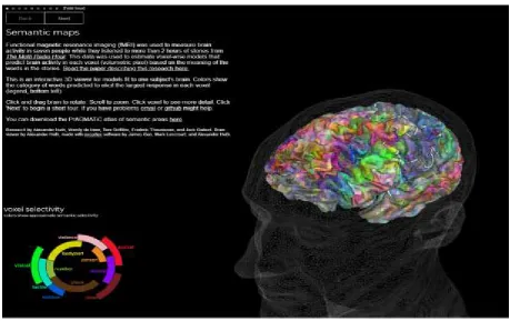
While the aforementioned studies investigated individual and separate areas of the brain that corresponded to semantics, a unified and comprehensive representation of semantic information across the cerebral system had not been done yet. In an effort to achieve this, Huth et. al (2016), mapped out the activity of cerebral blood-oxygen-level-dependent (BOLD) responses to different semantics. With the help of an fMRI machine, Huth and his colleagues captured the oxygen level response patterns in the participants’ brains while participants listened to stories of the “Moth Radio Hour”. Huth and his colleagues then, per activity pattern of the brain, mapped out the BOLD

responses per word spoken. A total of 10,470 words from the stories were embedded into four dimensions, using principal component analysis (PCA), within the semantic space. With these four dimensions, 11 distinct categories were identified using k-means clustering. The labels assigned to these categories were ‘numeric’, ‘visual’, ‘tactile’, ‘natural’, ‘temporal’, ‘violent’, ‘professional’, ‘mental’, ‘emotional’, ‘social’ and ‘communal’. This data is displayed on the website

https://gallanthub.org/huth2016, a screenshot of it can be seen below in figure 1.

Figure 1. Screenshot of Huth et. al's voxel wise modeling of the brain on https://gallantlab.org/huth2016/

6

1.2 The present study

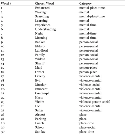
The present study hopes to supplement, and further shed light on the semantic system by comparing the categories created in Huth et. al (2016) study, with hand organized items of the same category by humans. With such general goals in mind, the present research is geared towards exploration, and is purely focused on finding patterns and differences between the items, categories created in Huth et. al (2016) and the categories that are sorted by humans when faced with the same items. Thus, the following research question is proposed: What are the similarities and differences between the way in which people categorize concepts, and the representation of concepts according to Huth et. al (2016)? In order to answer this question, a sample of 50 words are chosen from six of the categories, namely, ‘mental’, ‘person’, ‘violence’, ‘place’, ‘body part’ and ‘number’, from Huth et. al (2016) as shown below in table 1.

Table 1 All chosen words and corresponding category from Huth et. al (2016)

Word # Chosen Word Category

1 Exhausted mental-place-time

2 Waking mental

3 Searching mental-place-time

4 Learning mental

5 Experience mental-time

6 Understanding mental

7 Night mental-time

8 Morning mental-time

9 Banker person-social

10 Elderly person-social

11 Landlord person-social

12 Family person-social

13 Widow person-social

14 Sheriff person-social

15 Maid person-place

16 Owner person-place

17 Cruelty violence-mental

18 Evil violence-mental

19 Murder violence-social

20 Innocent violence-mental

21 Contempt violence-mental

22 Harm violence-mental

23 Victim violence-person-social

24 Die violence-mental

25 Suffer violence-mental

26 Airport place

27 Parking place

28 Lunch place-time

29 School place-social

7

31 Basement place

32 Attic place

33 Bedroom place

34 Male body part-person

35 Female body part-person

36 Breast body part-visual

37 Skull body part-visual

38 Chest body part-visual

39 Leg body part-number

40 Arm body part-number

41 Liver body part-violence-person

42 Five number

43 Ten number

44 Three number

45 Eight number

46 Reach number-place-visual

47 Onto number-place-visual

48 Miles number-outdoor

49 Set number

50 Distance number-outdoor-visual

All 50 items are written on separate paper cards without their categories, then, the cards were handed to participants who were further instructed to sort them into groups based on their personal opinion on how semantics is categorized. This simple technique is called ‘Hierarchical Card Sorting’, and can be used to elicit mental categorization and structure of different semantic domains.

A further 20 words were selected from the remaining semantic domains from Huth et. al (2016), namely, ‘social’, ‘time’, ‘outdoor’ and ‘visual’. These words will be assigned ‘false’ categories and mixed in with the aforementioned 50 words (that will be assigned their original categories). A questionnaire can then be created using the total 70 words and categories for participants to rate the word-categorical relatedness on a scale of one to five. The results can be used to analyze semantic relatedness between category and word, even if participants grouped them separately (due to reasons like, recall or multiple interpretations). The 20 ‘decoy’ questions can be used to see if participants answered the questions properly, as they are assigned false categories which should yield a higher (towards 5, meaning highly unrelated) average than all other items.

1.3 Hierarchical Card Sorting

8

predefined groups are provided by the researcher and participants are asked to sort the items into the predefined group that they see fit.

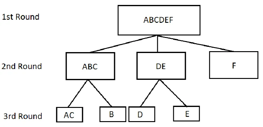
Card sorting’s precision and detail can be further improved using hierarchical cluster structures. By asking participants to further define subgroups in subsequent rounds (if applicable), the resulting distance score between items, or Jaccard Coefficient, is much more intricate (Faiks & Hyland, 2000).

Figure 1 three round hierarchical card sorting example

9

2. Methods

2.1 Participants

A total of 30 participants were recruited for the card sorting and questionnaire study, all participants were first, second or third year students studying at the University of Twente. 16

participants are male and 14 are female, ranging between ages 19-26 with an average age of 22 (SD = ± 3.4). A total of 12 participants are German, 11 are Dutch alongside seven internationals (Bulgarian, Romanian, Serbian, Norwegian, Irish, Brazilian and Italian). While all participants were able to speak English, most participants were not native speakers and did not linguistically understand one or two items. Nevertheless, most participants asked questions about items that they did not

recognize, and those who didn’t were prompted by the researcher to ensure full understanding. Thus, no participants were omitted for linguistic reasons. Finally, all participants were recruited through Sona-Systems and social media websites like Facebook, as well as through word of tell.

2.2 Materials

For the card sorting task, 50 paper cards were used to write the semantic terms needed for the study. The terms were handpicked from voxels in the 3D-voxel model of the brain on

http://gallantlab.org/huth2016. The criteria for selection were as follows: Firstly, terms were selected based on five categories that were chosen from Huth et. al (2016) 11 semantic categories, and a total of 50 words were selected from each category equally. Second, copies of words (e.g. see

and seeing) were avoided. Third, the voxels which the words are selected from must have a model performance (reliability) score of at least: Not bad, pretty reliable or better. Finally, voxels from both hemisphere (right and left) were selected for each category when possible, with its area (e.g. right-side prefrontal cortex) noted down.

For the questionnaire portion of the research, a questionnaire was constructed with two columns containing a word and the selected five categories for comparison. Next to each word comparison, a Likert Scale, ranging from 1-5, where 1 is “highly related” and 5 is “highly unrelated”. All 50 words used in the card sorting task are in the questionnaire, with their corresponding

10

2.3 Procedure

2.3.1 Briefing

Before beginning the study, each participant is given a written consent form and with an explanation of their right to withdraw from the study at any point during the study, and the chance to ask any questions during and after the study. Additionally, the privacy and use of their data, both card sorting and demographics, are disclosed and explained. Due to the potential effect of priming, a brief explanation of the study is given without any reference to Huth et. al, and a chance for elaboration is offered during the debriefing.

Participants are instructed to lay out the given 50 cards in clusters according to their own assessment, with the only rule being that it had to be semantically, instead of syntactically, based categories. Once the participants are satisfied with the groups, they are asked to further subdivide the groups, if they deem appropriate. Groups are no longer allowed to be mixed or re-arranged. Once participants are satisfied, they are asked again to, voluntarily, further subdivide the subgroups. In order to capture the card sort results, pictures were taken with a smartphone after each round. Finally, after the card sorting task is completed, participants are asked to fill in the questionnaire with a brief explanation of the layout.

2.4 Data Analysis: Questionnaire

11

Figure 2 vector analysis item vector examples with fruits

2.5 Data Analysis: Card Sorting

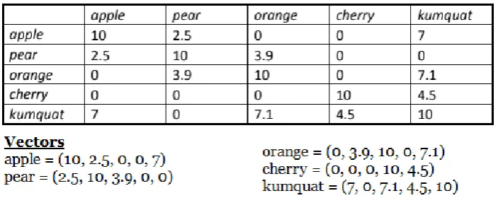
The collected data from the card sort are entered into excel spreadsheets on a 50x50 grid to display the Jaccard Coefficients, between each item. Jaccard Coefficient is calculated by dividing the number of groups which both items belong in with the number of groups either item belongs in.

To further process this result, Vector Analysis is used instead of the standard hierarchical cluster analysis, due to its increased precision, to create the item order for the heat map in R-studio. Vector analysis considers, on top of the highest score shared between two items, all other items that both items have in common. That is, the more common Jaccard scores the two items share with one another, the closer the distance. Since all scores of both items are compared, the two rows or

columns of values (The scores of each item with other items) can be seen as vectors, as shown below in figure 4.

These vectors can then be subtracted from one another, squared and summed to show the variance. Finally, the square root of the sum is taken to calculate the Euclidian distance score. The example below shows the Euclidian distance formula used between apple and pear:

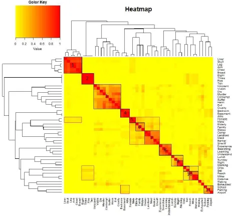
The distance scores between the items are then used as the basis for the dendrogram/heat map. The lower the Euclidian distance is, the stronger the relationship between vectors (more similar scores between the two items). The heat map visually displays the relationship between two items through a colouring spectrum of yellow to red, where red is an indication of high relation and yellow of low relation. Once the heat map is constructed, clusters can be justified as elicited mental categories based on the redness, or warmth, of the cluster with the support of logic and reasoning.

12

3. Results

3.1 Card Sorting

The finalized heat map is shown below in figure 1, structured with vector analysis and the scores colour coded with the ranges of yellow to red, between zero and one, respectively. The dark red squares represent items that are close (one) in terms of semantic distance, whereas the yellower squares represent a larger (zero) distance between items. From the heat map, clusters of red and dark orange squares are bordered in black as shown in figure 5. These clusters were decided based on how distinctively towards the spectrum of red they are compared to their surroundings.

13

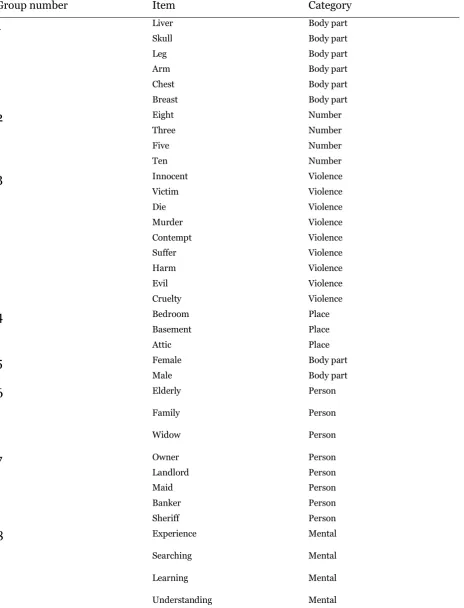
A total of 11 clusters could be created from the heat map, leaving two items as singletons. In clusters nine and ten, there are distinct subgroups represented by the darker regions of each groups as shown and bordered in figure 5. The items, their respective category and group number are shown below in Table 2.

Table 2 Cluster groups, items and categories

Group number Item Category

1

Skull Body part

Leg Body part

Arm Body part

Chest Body part

Breast Body part

2

Three Number

Five Number

Ten Number

3

Victim Violence

Die Violence

Murder Violence

Contempt Violence

Suffer Violence

Harm Violence

Evil Violence

Cruelty Violence

4

Basement Place

Attic Place

5

Male Body part

6

Family Person

Widow Person

7

Landlord Person

Maid Person

Banker Person

Sheriff Person

8

Searching Mental

Learning Mental

14

9

Night Mental-Time

Morning Mental-Time

10

Miles Number

Distance Number

Set Number

Onto Number

11

Parking Place

Airport Place

Singles Waking Mental

Exhausted Mental

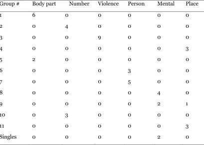
Table 3 Matrix showing number of items within each category per group from heat map

Group # Body part Number Violence Person Mental Place

1 6 0 0 0 0 0

2 0 4 0 0 0 0

3 0 0 9 0 0 0

4 0 0 0 0 0 3

5 2 0 0 0 0 0

6 0 0 0 3 0 0

7 0 0 0 5 0 0

8 0 0 0 0 4 0

9 0 0 0 0 2 1

10 0 3 0 0 0 0

11 0 0 0 0 0 3

Singles 0 0 0 0 2 0

15

Cluster three contains all of the items corresponding to the category ‘Violence’, although not all distance scores were very high. Scores between ‘Cruelty’, ‘Evil’, ‘Harm’, ‘Murder’ and ‘Suffer’ were significantly higher compared to the remaining cluster. Specifically, the item ‘Contempt’ did not score very well with many of the items in cluster three, likely due to the more advanced, and less acute nature of the word. When semantically compared to the other items (suffer, murder, etc.), the item ‘Contempt’ is much further from the extremity that is the category ‘Violence’. Additionally, insufficient vocabulary among participants will also contribute to the lack of connection, which is evident in the amount of participants who asked for the meaning of the word during the card sort. Lastly, the items ‘Victim’, ‘Die’ and ‘Murder also formed a distinct sub-cluster, likely because all items can often be found present in the same semantic context, that of a murder.

Cluster four contained the items ‘Bedroom’, ‘Basement’ and ‘Attic’, which are all rooms within a home. Cluster five contains the item ‘Male’, and its logical counterpart, ‘Female’. The sixth and seventh cluster both contain the items from the category ‘Person’. Cluster six has ‘Elderly’, ‘Family’ and ‘Widow’, which are all family and home related, whereas cluster seven contains more ‘general’ personell, like ‘Sheriff’ or ‘Banker’. Distinctly stronger scores can also be observed between the items ‘Owner’ and ‘Landlord’, and ‘Banker’ and ‘Sheriff’. Cluster eight contains the items

‘Experience’, ‘Searching’ and ‘Learning’, which are all mental processes involved with one another.

Cluster nine contains the items ‘Night’, ‘Morning’, ‘Lunch’ and ‘Sunday’, which represent time constructs. However, a stronger connection between ‘Night’ and ‘Morning’ can be observed. This is likely due to the two items being counterparts of one another, and are more related to time of the day, rather than day of the week like ‘Sunday’. This is further evident in their weak, but stronger connection with the item ‘Lunch’, which can also be interpreted as time of the day.

The tenth cluster contains the remaining ‘Number’ related items, though a gap exists

16

3.2 Questionnaire

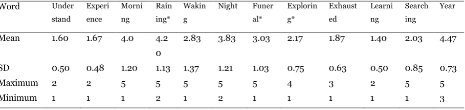
The means from the questionnaire are divided according to the six clusters chosen from Huth et. al (2016). A cut off score of 2.5 is chosen to determine whether the relation is relevant or not. This score represents the minimum on a scale of one to five (one is highly related, three is neutral and five is highly unrelated) where a concept becomes relevant with a category. In the following tables, all items and their mean scores are displayed along with the standard deviation (SD), maximum and minimum scores. The asterisk next to the words is an indication of filler word.

Table 4 Questionnaire item means corresponding to the category 'body part'

Word Female Chest Breast Leg Male Skull Garment* Aunt* Weekend* Arm Liver

Mean 2.97 1.20 1.03 1.03 3.07 1.30 3.57 4.60 4.77 1.03 1.20

SD 1.30 0.41 0.18 0.18 1.20 0.65 1.10 0.77 0.63 0.18 0.48

Maximum 5 2 2 2 5 4 5 5 5 2 3

Minimum 1 1 1 1 1 1 2 2 2 1 1

In table 4, the category corresponding to the words are ‘body part’. All three filler words had high mean scores and low standard deviation, indicating that the large majority of participants found these items to be irrelevant to the category (which means that participants are alert).

However, the filler word ‘garment’ had a slightly lower mean, most likely because garments are worn on body parts. The remaining items all scored equally low, ranging from a mean of 1.03 to 1.30 and all with a standard deviation of lower than 1.10. The two exceptions to the case are the items ‘male’ and ‘female’ which both scored a similar score of 3.07 and 2.97 respectively. Likely, participants understood that female and male refer also to genitalia differences, however, are much less specific towards ‘body parts’ than items like ‘arm’ or leg’.

Table 5 Questionnaire item means corresponding to the category 'mental'

Word Under

stand Experi ence Morni ng Rain ing* Wakin g

Night Funer al* Explorin g* Exhaust ed Learni ng Search ing Year

Mean 1.60 1.67 4.0 4.2

0

2.83 3.83 3.03 2.17 1.87 1.40 2.03 4.47

SD 0.50 0.48 1.20 1.13 1.37 1.21 1.03 0.75 0.63 0.50 0.85 0.73

Maximum 2 2 5 5 5 5 5 4 3 2 5 5

17

Items in table 5 correspond to the category ‘mental’. Two of the filler items had high mean scores, however, the item ‘exploring’ had a mean score of 2.17, which should be considered

significant. Although the item was originally drawn from the category of ‘outdoor’, it is easy to see why participants rated them to be semantically similar, as mental exploration is often used as a metaphor when engaging different cognitive processes. Aside from ‘morning’, ‘night’ and ‘year’, all other items scored significantly, between 1.40 and 2.03 with standard deviation between 0.48 and 0.85. The items ‘morning’, ‘night’ and ‘year’ are more likely considered to be related to time, which Huth and his colleagues consider mental, thus explaining why they scored insignificantly. These items also had a higher standard deviation, ranging from 0.73 to 1.20 and shows that some participants still considered them neutral or even slightly relevant.

Table 6 Questionnaire item means corresponding to the category 'number'

Word Three Eight Onto Ten Moonlight* Set Coat* Reach Five Miles Distance

Mean 1.13 1.03 4.40 1.03 4.87 2.67 4.57 3.83 1.00 2.33 2.00

SD 0.73 0.18 0.89 0.18 0.43 1.06 0.82 1.12 0.00 1.00 0.69

Maximum 5 2 5 2 5 5 5 5 1 5 4

Minimum 1 1 2 1 3 1 2 1 1 1 1

Table 6 contains all items corresponding to the category ‘number’. The two filler items ‘moonlight’ and ‘coat’ both had high mean scores of 4.87 and 4.57 respectively, with low standard deviation. This again indicates that the filler items worked and participants were paying properly doing the questionnaire. The remaining items scored varyingly. All of the literal number items scored between 1.00 and 1.13 (one participant chose five for the item ‘three’, which was likely a miss input) with low standard deviation between 0.00 – 0.18 (0.73 if counting ‘three’). ‘Miles’ and

‘distance’ scored 2.33 and 2.00 respectively, likely because while both items can be measured with numbers, are not necessarily completely numbers related, it could also be travelling related, for example. The item ‘set’ scored barely above the cut off line of 2.67, because while it is often used in a number related context, it is also commonly used in other contexts like preposition, or theatrics. Finally, ‘onto’ and ‘reach’ both have a high mean scores of 4.40 and 3.83 respectively, which shows that participants did not find them relatable to numbers. This is likely because participants do not see positional words like ‘onto’ or ‘reach’ as number related, however, they are spatially related which can also be number related (e.g. vectors).

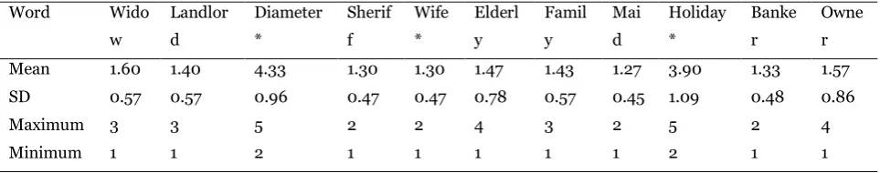
Table 7 Questionnaire item means corresponding to the category 'person'

Word Wido

w Landlor d Diameter * Sherif f Wife * Elderl y Famil y Mai d Holiday * Banke r Owne r

Mean 1.60 1.40 4.33 1.30 1.30 1.47 1.43 1.27 3.90 1.33 1.57

SD 0.57 0.57 0.96 0.47 0.47 0.78 0.57 0.45 1.09 0.48 0.86

Maximum 3 3 5 2 2 4 3 2 5 2 4

18

Table 7 contains all items corresponding to the category ‘person’. Aside from the item ‘wife’, understandably, all other filler items had a high mean score between 3.90-4.33 and low standard deviation. The filler word wife was chosen from the ‘social’ category, which can often overlap with the ‘person’ category as socializing often involves people. The remaining words all scored under the cut-off point, between 1.27 and 1.47 with low standard deviation, showing that participants found all items highly related.

Table 8 Questionnaire item means corresponding to the category 'place'

Word Scen

ery* Airpo rt Halfwa y* Hom e* Bedroo m Sund ay Baseme nt Days * Scho ol Park ing

Attic Lunc h Mean 1.73 1.50 1.37 3.10 1.53 4.40 1.37 4.37 1.30 1.67 1.33 3.93

SD 0.83 0.68 0.49 0.96 0.73 0.81 0.61 0.89 0.47 0.76 0.48 0.83

Maximum 4 3 2 5 4 5 3 5 2 3 2 5

Minimum 1 1 1 1 1 3 1 2 1 1 1 2

Table 8 contains all items corresponding to the category ‘place’. Surprisingly, all filler items have mean scores between very low and neutral, however, upon further inspection, it is clear as to why that is. The items ‘scenery’, ‘home’ and ‘halfway’ can all be easily related to the category ‘place’, since they all involve a physical place. The only filler item that scores highly is ‘days’, and is a word that is much less semantically related to ‘place’. The heat map items, aside from ‘lunch’, all scored significantly below the cut off score, ranging between 1.30 to 1.67, showing that participants found them to be highly related. ‘Lunch’ on the otherhand, while usually involving a place to sit or stand to eat, is much more semantically related to other categories (perhaps food? Or time?), according to participants.

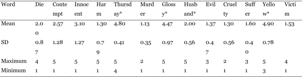
Table 9 Questionnaire item means corresponding to the category 'violence'

Word Die Conte

mpt Innoc ent Har m Thursd ay* Murd er Gloss y* Husb and*

Evil Cruel ty Suff er Yello w* Victi m

Mean 2.0

0

2.57 3.10 1.30 4.80 1.13 4.47 2.00 1.37 1.30 1.60 4.90 1.53

SD 0.8

7

1.28 1.27 0.7 9

0.41 0.35 0.97 0.56 0.4 7

0.56 0.4 0

0.78

Maximum 4 5 5 5 5 2 5 5 3 2 3 5 4

Minimum 1 1 1 1 4 1 1 1 1 1 1 3 1

19

meant that participants had varied opinions upon these items. This is likely because ‘contempt’ does not necessarily lead to violence, and while ‘innocent’ can be involved in violence, it is also an item that lies on the other end of the spectrum.

4. Discussion

The semantic categories established in Huth et al.’s (2016) study appear to be closely related to the results of the card sorting study, although some differences exist between them. Aside from cluster nine, all items within a cluster are categorically homogenous. In table 3, it can be observed that clusters one and five comprise of items from the ‘body part’ category, clusters two and ten have items from the ‘numbers’ category, clusters six and seven have items from the ‘person’ category, clusters eight and nine (aside from the item ‘sunday’) contains items from the ‘mental’ category, clusters 11 and four contains items from the ‘place’ category. Although not all items within cluster 11 were very close (as shown by the lighter, yellower patches), cluster 11 represents all the items from the ‘violence’ category from Huth et al. (2016). All of Huth and colleagues’ categories were split into two clusters except for ‘violence’, ‘mental’ and ‘place’. ‘Violence’ items were indicative enough to be grouped in one single cluster, however, ‘mental’ and ‘place’ had three separate clusters. This shows that the categories ‘mental’ and ‘place’ might be more interpretable than the remaining categories, which makes sense as the concept of ‘mental’ can be seen to be all encompassing (we interpret the world through our minds, which is mental, so the entire subjective interpretation of the world is ‘mental’), and ‘places’ can often involve different, more prominent contexts too (like places of your home, public/private places).

These categorical connections can also be observed in the heat map, for example, between clusters one and five, there is a distinctly darker yellow patch that represents weaker distance scores (denoted by the red borders in figure 5). These items were likely not grouped together as often due to the ambiguous nature of the items ‘Female’ and ‘Male’ and how it can be categorized with items of other categories like ‘Person’. This is further evident in the darker regions between clusters five, six and seven, despite the items from cluster five, being a part of the ‘Body part’ category rather than that of ‘Person’ from the items in clusters six and seven. The same observations can be made between clusters two and ten, six and seven, 11 and four, where all pairs share items of the same category from Huth et al. (2016). These observations provide some evidence and support for the categories created by Huth et al. (2016).

The differences between them can be attributed to many different possible factors. For one, it appears that, when confronted with the splitting (round two and three) portion of the card sort, participants are more likely to target larger groups, and split them based on more intricate

20

robbers). Likewise, ‘Victim’, ‘Die’ and ‘Murder’ from cluster three are all clustered together because a murder requires a victim, and a murder also requires a death, whereas other items in cluster three, like ‘Evil’ or ‘Suffer’, does not necessarily have to be involved in a murder. The same could be said for clusters ten and two. While both categories are numbers related, the literal number items from cluster two were much more distinctively relatable, and were thus more commonly grouped together. The items ‘Onto’ and ‘Set’ are both highly interpretable, and does not have to be number related (one could argue that ‘Onto’ is barely related to numbers), and were seldom grouped together with the rest of the number items. Since neuron activation is strengthened through repetition, it is likely that people have varying associations that is influenced by their past, and recent occurrences. For example, while most participants interpreted the item ‘Set’ from a theatrical or action domain, some participants grouped it with other numbers. These patterns also reflect the results of the questionnaire, for example, all of the ‘mental’ items that were grouped together on the heatmap (‘learning’, ‘experience’, ‘understanding’ and ‘searching’) scored significantly below the cut off score of 2.5, whereas the three items that were left out (‘night’, ‘morning’ and ‘waking) were all well above the cut off score. Another example is the category ‘body parts’, as participants

consistently rated all the ‘body part’ items significantly below the cut off score except for the items ‘female’ and ‘male’. On the heat map, ‘male’ and ‘female’ are also a distinct independent group that has little association with the rest of the ‘body part’ items. In the category of ‘numbers’, both ‘onto’, ‘set’ and ‘reach’, have high mean scores in comparison to the rest of the numbers. The exceptions are ‘miles’, ‘distance’, whom participants found to be rather related to numbers compared to during the card sort. These observations show that participants are fairly consistent across different methods of eliciting mental models, whether its card sorting or a questionnaire, and provide results that reflect upon one another.

There are a few explanations for the differences between the questionnaire, Huth et. al’s (2016) categories and the card sort categories. Firstly, due to the order of items, participants could activate different associations when confronted with the word ‘Set’ depending on the cards they encounter prior. Secondly, since all participants were university students, some participants who are studying in a more mathematical field may have a more active mathematical domain, and thus group ‘Set’ with other numbers. The human mind has the capability to create categories based on inconsistent criterions, whereas Huth et al.’s (2016) categories are generated based on consistency of semantic distance. It was a common occurrence that during the first round, participants created multiple smaller groups that might still be very related to other groups, instead of large

encompassing ones. This begs the question, whether these differences could be decreased if

participants were asked to create groups that had similar domain generality; and whether items like ‘miles’ and ‘distance’ would be grouped more often with the remaining numbers if that was the case.

21

participants for the card sorting, which lead to a variety of clustering methods. While some participants opted to slowly look through all cards before beginning to group them, others placed cards down and grouped them as they shuffled through the deck. Additionally, the disclosure of the second and third round group splitting only happened post first round, which meant that

participants often created multiple small groups and did not think generally enough to create bigger groups that could be further split. Lastly, many participants were non-native English speakers, and while some asked for clarification on unknown vocabulary, most participants required prompting before admitting that they did not understand an item. This is evident in the item ‘Contempt’, which is a fairly uncommonly used (amongst non-native speakers) synonym for hate. Some participants explained that they thought it was ‘Content’, while others wholly admitted to grouping it arbitrarily because they did not know what it meant.

Understanding how people categorize and associate semantic information is practically useful for a large variety of domains. In the learning sciences and education for example, such an information can be used to create and organize topic domains to help learners acquire the

information in an efficient and natural manner. The same principles could be applied to any environment in which semantic learning takes place, for example, when operating new tools or interactive machines. Designers would be able to create user goal relevant labels, more intuitive categorical lists that reduces user error in the face of inexperience. The card sorting technique has been applied in this manner in the past with varying results (Schmettow and Sommer, 2016)

5. Conclusion

The present study found clear relations between the categories from the semantic map constructed by Huth et al. (2016) and the card sorting results. Furthermore, most of the differences between the two can be reasoned with individual variations and methodological differences, like their method of sorting. Two of the six categories showed more variation and interpretability than others, namely, ‘place’ and ‘mental’. This suggests that some of the categories, like ‘mental’ and ‘place’, created by Huth and his colleagues may be a lot larger encompassing, and overlapping with other categories. Such a category is difficult to isolate in more mechanical and natural sorting methods like card sorting, where participants may not create such largely encompassing categories. While these items did not vary as greatly within the questionnaire, this is likely because of the semantically closed design of the questionnaire, where participants are forced to think about one relation between two items and that only.

22

(2016) more data-driven method creates more general, and consistently overlapping categories that can be considered all encompassing. These categories, or semantic domains, were decided based on statistical methods, and were thus only created to have similar semantic distance (vector based). The results of the present study suggest that the categories created by Huth and his colleagues’ data-driven methods of categorization are fairly representative of a human card sort using the same items. Although not all items that belongs to a category were together in one cluster, all items in a cluster were of the same category. Given the weak, but still relevant, distance scores that exist in the outskirts of the heat map, it can be concluded that most of these split categories still had

connections between them, and thus provide even further support for Huth’s categories.

23

6. Reference

Binder, J., Westbury, C., McKiernan, K., Possing, E., Medler, D. (2006). Distinct brain systems for processing concrete and abstract concepts. Journal of cognitive neuroscience, 17(6), 905-917. DOI: https://doi.org/10.1162/0898929054021102

Binder, J., Desai, H., Graves, W., & Conant, L. (2009). Where is the semantic system? A critical review and meta-analysis of 120 functional neuroimaging studies. Cerebral Cortex, 19(12), 2767–2796.

DOI: https://doi.org/10.1093/cercor/bhp055

Chertkow, H., Massoud, F., Nasreddine, Z., Belleville, S., Joanette, Y., Bocti, C., … Bergman, H. (2008). Diagnosis and treatment of dementia: 3. Mild cognitive impairment and cognitive impairment without dementia. CMAJ : Canadian Medical Association journal, 178(10), 1273– 1285. doi:10.1503/cmaj.070797

Damasio, H., Tranel, D., Grabowski, T., Adolphs, R., Damasio, A (2004). Neural systems behind word and concept retrieval. Cognition, 92(1-2), 179-229. DOI:

https://doi.org/10.1016/j.cognition.2002.07.001.

Dronkers, F., Wilkins, D., Van Valin, R., Redfern, B., Jaeger, J (2004). Lesion analysis of the brain areas invovled in language comprehension. Cognition 92(1-2), 145-177. DOI:

https://doi.org/10.1016/j.cognition.2003.11.002

Friederici, A., Opitz, B., Cramon, Y. (2000). Segregating semantic and syntactic aspects of

processing in the human brain: an fmri investigation of different word types. Cerebral Cortex, 10(7), 698-705.

DOI: https://doi.org/10.1093/cercor/10.7.698

Gainotti, G (2000). What the locus of brain lesion tells us about the nature of the cognitive defect underlying category-specific disorders: a review. Cortex, 36(4). 539-559. DOI:

https://doi.org/10.1016/S0010-9452(08)70537-9.

Hart, J.M., & Gordon, B. (1990). Delineation of single-word semantic comprehension deficits in aphasia, with anatomical correlation. Annals of neurology, 27(3), 226-31.

DOI: 10.1002/ana.410270303

Hillis, A. E., Wityk, R. J., Tuffiash, E. , Beauchamp, N. J., Jacobs, M. A., Barker, P. B. and Selnes, O. A. (2001), Hypoperfusion of Wernicke's area predicts severity of semantic deficit in acute stroke. Annals Neurology, 50, 561-566. doi:10.1002/ana.1265

Huth, A. G., De Heer, W. A., Griffiths, T. L., Theunissen, F. E., & Gallant, J. L. (2016). Natural speech reveals the semantic maps that tile human cerebral cortex. Nature, 532(7600), 453– 458.

DOI: https://doi.org/10.1038/nature17637

Mummery, C., Patterson, K., Price, J., Ashburner, J., Frackowiak, S. and Hodges, R. (2000). A voxel‐

based morphometry study of semantic dementia: relationship between temporal lobe atrophy and semantic memory. Annals of Neurology, 47, 36-45.

24

Rosch, E. (1975). Cognitive representations of semantic categories. Journal of experimental

psychology: General, 104(3), 192-233. DOI: http://dx.doi.org/10.1037/0096-3445.104.3.192

Tranel, D., Damasio, H. & Damasio, A.R (1997). A neural basis for the retrieval of conceptual knowledge. Neuropsychologia 35, 1319-1327. DOI: 10.1016/S0028-3932(97)00085-7.

Tulving, E. (1972). Episodic and Semantic Memory. In Organiz. Mem. Lon. (Vol. 381, pp. 381–403). Warrington, E., McCarthy, R (1983). Category specific access dysphasia. Brain, 106(4), 859-878.

DOI: https://doi.org/10.1093/brain/106.4.859

25

7. Appendices

Appendix A: Chosen stimulus item per category

Word # Chosen Word Category Voxel Location(Right or Left) Reliability

1 Exhausted mental-place-time 21,77,31 PL(R) 0.264

2 Waking mental 21,77,31 PL(R) 0.264

3 Searching mental-place-time 21,77,31 PL(R) 0.264

4 Learning mental 13,90,56 PL(L) 0.307

5 Experience mental-time 13,90,56 PL(L) 0.307

6 Understanding mental 13,90,56 PL(L) 0.307

7 Night mental-time 19,82,48 PL(R) 0.425

8 Morning mental-time 19,82,48 PL(R) 0.425

9 Banker person-social 24,27,40 FL(R) 0.305

10 Elderly person-social 24,27,40 FL(R) 0.305

11 Landlord person-social 26,35,43 FL(R) 0.349

12 Family person-social 14,81,73 PL(L) 0.333

13 Widow person-social 14,81,73 PL(L) 0.333

14 Sheriff person-social 15,81,29 PL(R) 0.41

15 Maid person-place 15,81,29 PL(R) 0.41

16 Owner person-place 15,81,29 PL(R) 0.41

17 Cruelty violence-mental 14,33,74 FL(L) 0.323

18 Evil violence-mental 14,33,74 FL(L) 0.323

19 Murder violence-social 14,33,74 FL(L) 0.323

20 Innocent violence-mental 24,25,54 FL(L) 0.309

21 Contempt violence-mental 24,25,54 FL(L) 0.309

22 Harm violence-mental 24,25,54 FL(L) 0.309

23 Victim violence-person-social 12,67,78 TL(L) 0.477

24 Die violence-mental 12,67,78 TL(L) 0.477

25 Suffer violence-mental 12,67,78 TL(L) 0.477

26 Airport place 15,89,61 OL(L) 0.359

27 Parking place 15,89,61 OL(L) 0.359

28 Lunch place-time 18,15,42 FL(R) 0.306

29 School place-social 18,15,42 FL(R) 0.306

30 Sunday place-time 18,15,42 FL(R) 0.306

31 Basement place 25,39,34 FL(R) 0.339

32 Attic place 25,39,34 FL(R) 0.339

33 Bedroom place 25,39,34 FL(R) 0.339

34 Male bodypart-person 21,40,72 FL(L) 0.273

35 Female bodypart-person 21,40,72 FL(L) 0.273

36 Breast bodypart-visual 16,35,69 FL(L) 0.286

37 Skull bodypart-visual 16,35,69 FL(L) 0.286

38 Chest bodypart-visual 14,29,66 FL(L) 0.222

39 Leg bodypart-number 14,29,66 FL(L) 0.222

26

41 Liver bodypart-violence?-person? 17,36,73 FL(L) 0.285

42 Five number 16,86,61 PL(L) 0.381

43 Ten number 16,86,61 PL(L) 0.381

44 Three number 16,86,61 PL(L) 0.381

45 Eight number 16,86,61 PL(L) 0.381

46 Reach number-place-visual 16,87,58 PL(L) 0.467

47 Onto number-place-visual 16,87,58 PL(L) 0.467

48 Miles number-outdoor 26,45,58 PL(L) 0.425

49 Set number 26,45,58 PL(L) 0.425

28

Appendix C: Questionnaire

Questionnaire: Relations

How do you judge the relation between these pairs of words on a scale of one to five?

Word 1 Word 2

1

2

3

4

5

Scenery place ⃝ ⃝ ⃝ ⃝ ⃝

Airport place ⃝ ⃝ ⃝ ⃝ ⃝

Three number ⃝ ⃝ ⃝ ⃝ ⃝

Female bodypart ⃝ ⃝ ⃝ ⃝ ⃝

Moonlight number ⃝ ⃝ ⃝ ⃝ ⃝

Eight number ⃝ ⃝ ⃝ ⃝ ⃝

Understanding mental ⃝ ⃝ ⃝ ⃝ ⃝

Breast bodypart ⃝ ⃝ ⃝ ⃝ ⃝

Exploring mental ⃝ ⃝ ⃝ ⃝ ⃝

Widow person ⃝ ⃝ ⃝ ⃝ ⃝

Coat number ⃝ ⃝ ⃝ ⃝ ⃝

Chest bodypart ⃝ ⃝ ⃝ ⃝ ⃝

Home place ⃝ ⃝ ⃝ ⃝ ⃝

Landlord person ⃝ ⃝ ⃝ ⃝ ⃝

Male bodypart ⃝ ⃝ ⃝ ⃝ ⃝

Leg bodypart ⃝ ⃝ ⃝ ⃝ ⃝

Die violence ⃝ ⃝ ⃝ ⃝ ⃝

Onto number ⃝ ⃝ ⃝ ⃝ ⃝

Miles number ⃝ ⃝ ⃝ ⃝ ⃝

Diameter person ⃝ ⃝ ⃝ ⃝ ⃝

Experience mental ⃝ ⃝ ⃝ ⃝ ⃝

Contempt violence ⃝ ⃝ ⃝ ⃝ ⃝

Set number ⃝ ⃝ ⃝ ⃝ ⃝

Owner person ⃝ ⃝ ⃝ ⃝ ⃝

Halfway place ⃝ ⃝ ⃝ ⃝ ⃝

Bedroom place ⃝ ⃝ ⃝ ⃝ ⃝

Innocent violence ⃝ ⃝ ⃝ ⃝ ⃝

Harm violence ⃝ ⃝ ⃝ ⃝ ⃝

Sunday place ⃝ ⃝ ⃝ ⃝ ⃝

Sheriff person ⃝ ⃝ ⃝ ⃝ ⃝

Morning mental ⃝ ⃝ ⃝ ⃝ ⃝

Basement place ⃝ ⃝ ⃝ ⃝ ⃝

Banker person ⃝ ⃝ ⃝ ⃝ ⃝

Waking mental ⃝ ⃝ ⃝ ⃝ ⃝

Wife person ⃝ ⃝ ⃝ ⃝ ⃝

Thursday violence ⃝ ⃝ ⃝ ⃝ ⃝

Raining mental ⃝ ⃝ ⃝ ⃝ ⃝

29

Murder violence ⃝ ⃝ ⃝ ⃝ ⃝

Days place ⃝ ⃝ ⃝ ⃝ ⃝

Ten number ⃝ ⃝ ⃝ ⃝ ⃝

Glossy violence ⃝ ⃝ ⃝ ⃝ ⃝

Five number ⃝ ⃝ ⃝ ⃝ ⃝

Holiday person ⃝ ⃝ ⃝ ⃝ ⃝

Aunt bodypart ⃝ ⃝ ⃝ ⃝ ⃝

Garment bodypart ⃝ ⃝ ⃝ ⃝ ⃝

Elderly person ⃝ ⃝ ⃝ ⃝ ⃝

Husband social ⃝ ⃝ ⃝ ⃝ ⃝

Maid person ⃝ ⃝ ⃝ ⃝ ⃝

Evil violence ⃝ ⃝ ⃝ ⃝ ⃝

Cruelty violence ⃝ ⃝ ⃝ ⃝ ⃝

Arm bodypart ⃝ ⃝ ⃝ ⃝ ⃝

Funeral mental ⃝ ⃝ ⃝ ⃝ ⃝

Suffer violence ⃝ ⃝ ⃝ ⃝ ⃝

Yellow violence ⃝ ⃝ ⃝ ⃝ ⃝

School place ⃝ ⃝ ⃝ ⃝ ⃝

Parking place ⃝ ⃝ ⃝ ⃝ ⃝

Weekend bodypart ⃝ ⃝ ⃝ ⃝ ⃝

Reach number ⃝ ⃝ ⃝ ⃝ ⃝

Night mental ⃝ ⃝ ⃝ ⃝ ⃝

Distance number ⃝ ⃝ ⃝ ⃝ ⃝

Attic place ⃝ ⃝ ⃝ ⃝ ⃝

Lunch place ⃝ ⃝ ⃝ ⃝ ⃝

Victim violence ⃝ ⃝ ⃝ ⃝ ⃝

Family person ⃝ ⃝ ⃝ ⃝ ⃝

Liver bodypart ⃝ ⃝ ⃝ ⃝ ⃝

Learning mental ⃝ ⃝ ⃝ ⃝ ⃝

Exhausted mental ⃝ ⃝ ⃝ ⃝ ⃝

Year mental ⃝ ⃝ ⃝ ⃝ ⃝

30

Appendix D: R-scripts for averaging all scores

setwd("c:/Users/Gebruiker/Desktop/Bachelor Thesis/Participant Data/Processed data")

available_files <- list.files(pattern = ".csv")

total <- matrix(nrow = 50, ncol = 50, data = rep(0, 2500))

for(f in 1:length(available_files)){

tab <- read.csv(available_files[f], stringsAsFactors = F)

tab <- tab[2:nrow(tab), 3:ncol(tab)]

#tab <- tab[1:50,]

# tab <- as.matrix(tab)

for (c in 1:ncol(tab)) {

tab[,c] <- as.numeric(tab[,c])

}

total <- total + tab

}

total <- total / length(available_files)

31

Appendix E: R-scripts for vector analysis and heat map

library(gplots)

library(RColorBrewer)

#Read the data file (.csv format)

data <- read.csv("c:/Users/Gebruiker/Desktop/Bachelor Thesis/Participant Data/Processed data.finaldata.csv")

# Transform data in numerical format

mat_data <- data.matrix(data[,1:ncol(data)])

# Define colors of heatmap: red for high numbers

my_palette <- colorRampPalette(c("yellow","red"))(n = 299)

# Call heatmap function (from gplots), with these arguments

# See:

https://www.rdocumentation.org/packages/gplots/versions/3.0.1/topics/heatmap.2

# Note: argument 'main=' gives name of plot

heatmap.2(mat_data, col = my_palette, density.info="none", trace="none",