warwick.ac.uk/lib-publications
Original citation:
Ottobre, Michela, Pillai, Natesh S., Pinski, Frank J. and Stuart, Andrew M.. (2015) A function
space HMC algorithm with second order Langevin diffusion limit. Bernoulli, 22 (1). pp.
60-106.
Permanent WRAP URL:
http://wrap.warwick.ac.uk/86355
Copyright and reuse:
The Warwick Research Archive Portal (WRAP) makes this work of researchers of the
University of Warwick available open access under the following conditions. Copyright ©
and all moral rights to the version of the paper presented here belong to the individual
author(s) and/or other copyright owners. To the extent reasonable and practicable the
material made available in WRAP has been checked for eligibility before being made
available.
Copies of full items can be used for personal research or study, educational, or not-for-profit
purposes without prior permission or charge. Provided that the authors, title and full
bibliographic details are credited, a hyperlink and/or URL is given for the original metadata
page and the content is not changed in any way.
Publisher’s statement:
http://projecteuclid.org/euclid.bj/1443620844
A note on versions:
The version presented in WRAP is the published version or, version of record, and may be
cited as it appears here.
DOI:10.3150/14-BEJ621
A function space HMC algorithm with
second order Langevin diffusion limit
M I C H E L A OT TO B R E1, NAT E S H S . P I L L A I2, F R A N K J . P I N S K I3and
A N D R E W M . S T UA RT4
1Department of Mathematics, Imperial College, 180 Queen’s Gate, SW7 2AZ, London, UK.
E-mail:[email protected]
2Department of Statistics, Harvard University, 1 Oxford Street, Cambridge, MA 02138, USA.
E-mail:[email protected]
3Department of Physics, University of Cincinnati, P.O. Box 210011, Cincinnati, OH 45221-0377, USA.
E-mail:[email protected]
4Mathematics Institute, Warwick University, CV4 7AL, UK. E-mail:[email protected]
We describe a new MCMC method optimized for the sampling of probability measures on Hilbert space which have a density with respect to a Gaussian; such measures arise in the Bayesian approach to inverse problems, and in conditioned diffusions. Our algorithm is based on two key design principles: (i) algo-rithms which are well defined in infinite dimensions result in methods which do not suffer from the curse of dimensionality when they are applied to approximations of the infinite dimensional target measure on RN; (ii) nonreversible algorithms can have better mixing properties compared to their reversible counter-parts. The method we introduce is based on the hybrid Monte Carlo algorithm, tailored to incorporate these two design principles. The main result of this paper states that the new algorithm, appropriately rescaled, converges weakly to a second order Langevin diffusion on Hilbert space; as a consequence the algorithm explores the approximate target measures onRNin a number of steps which is independent ofN. We also present the underlying theory for the limiting nonreversible diffusion on Hilbert space, including charac-terization of the invariant measure, and we describe numerical simulations demonstrating that the proposed method has favourable mixing properties as an MCMC algorithm.
Keywords:diffusion limits; function space Markov chain Monte Carlo; hybrid Monte Carlo algorithm; second order Langevin diffusion
1. Introduction
Markov chain Monte Carlo (MCMC) algorithms for sampling from high dimensional probability distributions constitute an important part of Bayesian statistical inference. This paper is focussed on the design and analysis of such algorithms to sample a probability distribution on an infinite dimensional Hilbert spaceHdefined via a density with respect to a Gaussian; such problems arise in the Bayesian approach to inverse problems (or Bayesian nonparametrics) [21] and in the theory of conditioned diffusion processes [9]. Metropolis–Hastings algorithms [10] constitute a popular class of MCMC methods for sampling an arbitrary probability measure. They proceed by constructing an irreducible,reversibleMarkov chain by first proposing a candidate move and then accepting it with a certain probability. The acceptance probability is chosen so as to preserve the detailed balance condition ensuring reversibility. In this work, we build on the generalized
Hybrid Monte Carlo (HMC) method of [11] to construct a newnonreversibleMCMC method appropriate for sampling measures defined via density with respect to a Gaussian measure on a Hilbert space. We also demonstrate that, for a particular set of parameter values in the algorithm, there is a natural diffusion limit to the second order Langevin (SOL) equation with invariant measure given by the target. We thus name the new method the SOL-HMC algorithm. Our con-struction is motivated by the following two key design principles:
1. designing proposals which are well-defined on the Hilbert space results in MCMC meth-ods which do not suffer from the curse of dimensionality when applied to sequences of approximating finite dimensional measures onRN;
2. nonreversible MCMC algorithms, which are hence not from the Metropolis–Hastings class, can have better sampling properties in comparison with their reversible counterparts.
The idea behind the first principle is explained in [6] which surveys a range of algorithms de-signed specifically to sample measures defined via a density with respect to a Gaussian; the unifying theme is that the proposal is reversible with respect to the underlying Gaussian so that the accept–reject mechanism depends only on the likelihood function and not the prior distribu-tion. The second principle above is also well-documented: nonreversible Markov chains, often constructed by performing individual time-reversible1steps successively [12,13], or by building
on Hamiltonian mechanics [7,11,15], may have better mixing properties.
Since the target distribution has support on an infinite dimensional space, practical implemen-tation of MCMC involves discretizing the parameter space, resulting in a target measure onRN, withN1. It is well known that such discretization schemes can suffer from the curse of di-mensionality: the efficiency of the algorithm decreases as the dimensionN of the discretized space grows large. One way of understanding this is through diffusion limits of the algorithm. In the context of measures defined via density with respect to Gaussian, this approach is taken in the papers [14,18] which show that the random walk Metropolis and Langevin algorithms requireO(N ) andO(N1/3)steps respectively, to sample the approximating target measure in RN. If, however, the algorithm is defined on Hilbert space then it is possible to explore the tar-get inO(1)steps and this may also be demonstrated by means of a diffusion limit. The paper [17] uses this idea to study a Metropolis–Hastings algorithm which is defined on Hilbert space and is a small modification of the random walk Metropolis method; the diffusion limit is a first order reversible Langevin diffusion. Moreover the diffusion limits in [14,18] are derived under stationarity whereas the results in [18] hold foranyinitial condition. The above discussion has important practical consequences: as implied by the above diffusion limits, algorithms which are well defined on the function spaces show an order of magnitude improvement in the mixing time in these high dimensional sampling problems.
Here we employ similar techniques as that of [17] to study our new nonreversible MCMC method, and show that, after appropriate rescaling, it converges to a second order nonreversible Langevin diffusion. Our new algorithm is inspired by similar algorithms in finite dimensions, starting with the work of [11], who showed how the momentum updates could be correlated in the original HMC method of [8], and the more recent work [5] which made the explicit connection to second order Langevin diffusions; a helpful overview and discussion may be found in [15].
Diffusion limit results similar to ours are proved in [4,5] for finite dimensional problems. In those papers, an accept–reject mechanism is appended to various standard integrators for the first and second order Langevin equations, and shown not to destroy the strong pathwise convergence of the underlying methods. The reason for this is that rejections are rare when small time-steps are used. The same reasoning underlies the results we present here, although we consider an infinite dimensional setting and use only weak convergence. Another existing work underpinning that presented here is the paper [2] which generalizes the hybrid Monte Carlo method for measures defined via density with respect to a Gaussian so that it applies on Hilbert space. Indeed the algorithm we introduce in this paper includes the one from [2] as a special case and uses the split-step (non-Verlet) integrator first used there. The key idea of the splitting employed is to split according to linear and nonlinear dynamics within the numerical Hamiltonian integration step of the algorithm, rather than according to position and momentum. This allows for an algorithm which exactly preserves the underlying Gaussian reference measure, without rejections, and is key to the fact that the methods are defined on Hilbert space even in the non-Gaussian case.
We now define the class of models to which our main results are applicable. Letπ0 andπ
be two measures on a Hilbert space (H,·,·, · )and assume that π0 is Gaussian so that
π0=N(0, C), withC a covariance operator. The target measureπ is assumed to be absolutely
continuous with respect toπ0and given by the identity
dπ
dπ0
(x)=Mexp
−(x), x∈H (1.1)
for a real valued functional(which denotes the negative log-likelihood in the case of Bayesian inference) andM a normalizing constant. Although the above formulation may appear quite abstract, we emphasize that this points to the wide-ranging applicability of our theory: the setting encompasses a large class of models arising in practice, including nonparametric regression using Gaussian random fields and statistical inference for diffusion processes and bridge sampling [9, 21].
In Section 2, we introduce our new algorithm. We start in a finite dimensional context and then explain parametric choices made with reference to the high or infinite dimensional setting. We demonstrate that various other algorithms defined on Hilbert space, such as the function space MALA [3] and function space HMC algorithms [2], are special cases. In Section3, we describe the infinite dimensional setting in full and, in particular, detail the relationship between the change of measure, encapsulated in, and the properties of the Gaussian priorπ0. Section4
contains the theory of the SPDE which both motivates our class of algorithms, and acts as a limit-ing process for a specific instance of our algorithm applied on a sequence of spaces of increaslimit-ing dimensionN. We prove existence and uniqueness of solutions to the SPDE and characterize its invariant measure. Section5contains statement of the key diffusion limit Theorem5.1. Whilst the structure of the proof is outlined in some detail, various technical estimates are left for Ap-pendicesAandB. Section6contains some numerics illustrating the new algorithm in the context of a problem from the theory of conditioned diffusions. We make some brief concluding remarks in Section7.
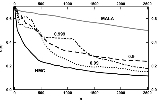
demonstrates that the method is comparable in efficiency to the function space HMC method in-troduced in [2] for a test problem arising in conditioned diffusions; until now, the function space HMC method was the clear best choice as demonstrated numerically in [2]. Furthermore, our numerical results indicate that for certain parameter choices in the SOL-HMC algorithm, and for certain target measures, we are able to improve upon the performance of the function space HMC algorithm, corroborating a similar observation made in [11] for the finite dimensional samplers that form motivation for the new family of algorithms that we propose here. From a technical point of view, the diffusion limit proved in this paper is similar to that proved for the function space MALA in [18], extending to the nonreversible case; however significant technical issues arise which are not present in the reversible case and, in particular, incorporating momentum flips into the analysis, which occur for every rejected step, requires new ideas.
2. The SOL-HMC algorithm
In this section, we introduce the SOL-HMC algorithm studied in this paper. We first describe the basic ideas from stochastic dynamics underlying this work, doing so in the finite dimensional setting ofH=RN, i.e., when the target measureπ(q)is a probability measure onRN of the form
dπ
dπ0
(q)∝exp−(q),
whereπ0 is a mean zero Gaussian with covariance matrix C and(q) is a function defined
onRN. A key idea is to work with an extended phase space in which the original variables are viewed as ‘positions’ and then ‘momenta’ are added to complement each position. We then ex-plain the advantages of working with ‘velocities’ rather than ‘momenta’, in the large dimension limit. And then finally we introduce our proposed algorithm, which is built on the measure pre-serving properties of the second order Langevin equation. As already mentioned, our algorithm will build on some basic facts about Hamiltonian mechanics. For a synopsys about the Hamilto-nian formalism see AppendixC.
2.1. Measure preserving dynamics in an extended phase space
Introduce the auxiliary variablep (‘momentum’) andMa user-specified, symmetric positive definite ‘mass’ matrix. Let0denote the Gaussian onR2N defined as the independent product of GaussiansN (0,C)andN (0,M)on theqandpcoordinates, respectively, and defineby
d
d0(q, p)∝exp
−(q).
A key point to notice is that the marginal of(q, p)with respect toq is the target measure
π(q). Define the Hamiltonian inH:R2N→Rgiven by
whereL=C−1. The corresponding canonical Hamiltonian differential equation is given by
dq
dt = ∂H
∂p =M
−1p, dp
dt = − ∂H
∂q = −Lq−D(q). (2.1)
This equation preserves any smooth function of H(q, p) and, as a consequence, the Liouville equation corresponding to (2.1) preserves the probability density of(q, p), which is propor-tional to exp(−H(q, p)). This fact is the basis for HMC methods [8] which randomly sample momentum from the GaussianN (0,M)and then run the Hamiltonian flow forT time units; the resulting Markov chain onq isπ(q)invariant. In practice, the Hamiltonian flow must be inte-grated numerically, but if a suitable integrator is used (volume-preserving and time-reversible) then a simple accept–reject compensation corrects for numerical error.
Define
z=
q p
and
J=
0 I −I 0
.
Then the Hamiltonian system can be written as
dz
dt =J DH(z), (2.2)
where, abusing notation,H(z):=H(q, p). The equation (2.2) preserves the measure. Now define the matrix
K=
K1 0
0 K2
,
where bothK1andK2are symmetric. The following SDE also preserves the measure:
dz
dt = −KDH(z)+ √
2KdW dt .
HereW=(W1, W2)denotes a standard Brownian motion onR2N. This SDE decouples into two
independent equations forq andp; the equation for q is what statisticians term the Langevin equation [18], namely
dq
dt = −K1
Lq+D(q)+2K1
dW1
dt ,
whilst the equation forpis simply the Ornstein–Uhlenbeck process:
dp
dt = −K2M
−1p+
2K2
dW2
Discretizing the Langevin equation (resp., the random walk found by ignoring the drift) and adding an accept–reject mechanism, leads to the Metropolis–Adjusted Langevin (MALA) (resp., the Random Walk Metropolis (RWM) algorithm).
A natural idea is to try and combine benefits of the HMC algorithm, which couples the posi-tion and momentum coordinates, with the MALA and RWM methods. This thought experiment suggests considering the second order Langevin equation2
dz
dt =J DH(z)−KDH(z)+ √
2KdW
dt , (2.3)
which also preservesas a straightforward calculation with the Fokker–Planck equation shows.
2.2. Velocity rather than momentum
Our paper is concerned with using the equation (2.3) to motivate proposals for MCMC. In partic-ular, we will be interested in choices of the matricesM,K1andK2which lead to well-behaved
algorithms in the limit of largeN. To this end, we write the equation (2.3) in position and mo-mentum coordinates as
dq
dt =M
−1p−K
1
Lq+D(q)+2K1
dW1
dt ,
dp
dt = −
Lq+D(q)−K2M−1p+
2K2
dW2
dt .
In our subsequent analysis, which concerns the largeN limit, it turns out to be useful to work with velocity rather than momentum coordinates; this is because the optimal algorithms in this limit are based on ensuring that the velocity and position coordinates all vary on the same scale. For this reason, we introducev=M−1pand rewrite the equations as
dq
dt =v−K1
Lq+D(q)+2K1
dW1
dt ,
Mdv
dt = −
Lq+D(q)−K2v+
2K2
dW2
dt .
In the infinite dimensional setting, i.e., whenHis an infinite dimensional Hilbert space, this equation is still well posed (see (2.5) below and Theorem 4.1). However in this case W1 and
W2are cylindrical Wiener processes onH(see Section3.1) andL=C−1is necessarily an
un-bounded operator onHbecause the covariance operatorCis trace class onH. The unbounded operators introduce undesirable behaviour in the largeN limit when we approximate them; thus we chooseMand theKi to remove the appearance of unbounded operators. To this end, we
2Physicists often refer to this astheLangevin equation for the choiceK
1≡0 which leads to noise only appearing in the
setM=L=C−1,K1=1CandK2=2C−1and assume that1and2commute withCto
obtain the equations
dq
dt =v−1
q+CD(q)+21C
dW1
dt , (2.4a)
dv
dt = −
q+CD(q)−2v+
22C
dW2
dt , (2.4b)
or simply
dq
dt =v−1
q+CD(q)+21
dB1
dt , (2.5a)
dv
dt = −
q+CD(q)−2v+
22
dB2
dt . (2.5b)
In the above,B1andB2areH-valued Brownian motions with covariance operatorC. This
equa-tion is well-behaved in infinite dimensions provided that theiare bounded operators, and under natural assumptions relating the reference measure, via its covarianceC, and the log density, which is a real valued functional defined on an appropriate subspace ofH. Detailed definitions and assumptions regarding (2.5) are contained in the next Section3. Under such assumptions, the function
F (q):=q+CD(q) (2.6)
has desirable properties (see Lemma3.4), making the existence theory for (2.5) straightforward. We develop such theory in Section4– see Theorem4.1. Furthermore, in Theorem4.2we will also prove that equation (2.5) preserves the measure(dq,dv)defined by
d
d0
(q, v)∝exp−(q), (2.7)
where0is the independent product ofN (0,C)with itself. The measure(resp.,0) is simply
the measure (resp.,0) in the caseM=C−1and rewritten in(q, v)coordinates instead of
(q, p). In finite dimensions, the invariance of follows from the discussions concerning the invariance of.
2.3. Function space algorithm
We note that the choice1≡0 gives the standard (physicists) Langevin equation
d2q
dt +2
dq
dt +
q+CD(q)=22C
dW2
dt . (2.8)
equation (2.9) below. In the finite dimensional setting, a method closely related to the one that we introduce was proposed in [11]; however we will introduce different Hamiltonian solvers which are tuned to the specific structure of our measure, in particular to the fact that it is defined via density with respect to a Gaussian. We will be particularly interested in choices of parameters in the algorithm which ensure that the output (suitability interpolated to continuous time) behaves like (2.8) whilst, as is natural for MCMC methods, exactly preserving the invariant measure. This perspective on discretization of the (physicists) Langevin equation in finite dimensions was introduced in [4,5].
In position/velocity coordinates, and using (2.6), (2.5) becomes
dq
dt =v,
(2.9) dv
dt = −F (q)−2v+
22C
dW2
dt .
The algorithm we use is based on splitting (2.9) into an Ornstein–Uhlenbeck (OU) process and a Hamiltonian ODE. The OU process is
dq
dt =0,
(2.10) dv
dt = −2v+
22C
dW2
dt ,
and the Hamiltonian ODE is given by
dq
dt =v,
(2.11) dv
dt = −F (q).
The solution of the OU process (2.10) is denoted by(q(t), v(t))=0(q(0), v(0);ξt); hereξtis
a mean zero Gaussian random variable with covariance operatorC(I−exp(−2t 2)). Notice that
the dynamics given by both (2.10) and by (2.11) preserve the target measure given in (2.7). This naturally suggests constructing an algorithm based on alternating the above two dynamics. However, note that whilst (2.10) can be solved exactly, (2.11) requires a further numerical ap-proximation. If the numerical approximation is based on a volume-preserving and time-reversible numerical integrator, then the accept–reject criterion for the resulting MCMC algorithm can be easily expressed in terms of the energy differences inH. A flowϕt onR2N is said to be time-reversible ifϕt(q(0), v(0))=(q(t), v(t))impliesϕt(q(t),−v(t ))=(q(0),−v(0)). Defintion of time-reversible and discussion of the roles of time-reversible and volume-preserving integrators may be found in [20].
leads to an algorithm which is exact (no rejections) in the purely Gaussian case where≡0. The splitting method proposed in [2] is via the linear and nonlinear parts of the problem, leading us to consider the two equations
dq
dt =v,
dv
dt = −q, (2.12)
with solution denoted as(q(t), v(t))=Rt(q(0), v(0)); and
dq
dt =0,
dv
dt = −CD(q), (2.13)
with solution denoted as(q(t), v(t))=t1(q(0), v(0)). We note that the map
χt=t /12◦Rt◦t /12
is a volume-preserving and time-reversible second order accurate approximation of the Hamilto-nian ODE (2.11). We introduce the notation
χτt =χt◦ · · · ◦χt, τ t
times
to denote integration, using this method, up to timeτ. This integrator can be made to preserve the measureif appended with a suitable accept–reject rule as detailed below. On the other hand the stochastic mapt0preservessince it leavesqinvariant and since the OU process, which is solved exactly, preserves0. We now take this idea to define our MCMC method. The infinite
dimensional Hilbert spaceHs ×Hs in which the chain is constructed will be properly defined in the next section. Here we focus on the algorithm, which will be explained in more details and analyzed in Section5.
Define the operationso thatvis the velocity component ofδ0(q, v). The preceding consid-erations suggest that from point(q0, v0)∈Hs×Hs we make the proposal
q∗1, v∗1=χτh◦δ0q0, v0
and that the acceptance probability is given by
αx0, ξδ:=1∧expHq0,v0−Hq∗1, v∗1,
where
H(q, v)=12q,C−1q+12v,C−1v+(q), (2.14) ·,·denoting scalar product inH. One step of the resulting MCMC method is then defined by setting
q1, v1=q∗1, v∗1 with probabilityαx0, ξδ
We will make further comments on this algorithm and on the expression (2.14) for the Hamilto-nian in Section5, see Remark5.6. Here it suffices simply to note that whilstH will be almost surely infinite, the energy difference is well-defined for the algorithms we employ. We stress that when the proposal is rejected the chain does not remain in(q0, v0)but it moves to(q0,−(v0)); i.e., the position coordinate stays the same while the velocity coordinate is first evolved according to (2.10) and then the sign is flipped. This flipping of the sign, needed to preserve reversibility, leads to some of the main technical differences with respect to [17]; see Remark5.13. For the finite dimensional case with Verlet integration the form of the accept–reject mechanism and, in particular, the sign-reversal in the velocity, was first derived in [11] and is discussed in further de-tail in Section 5.3 of [15]. The algorithm (2.15) preservesand we refer to it as the SOL-HMC algorithm. Recalling thatvdenotes the velocity component ofδ0(q, v), we can equivalently use the notationsα(x, ξδ)andα(q, v), forx=(q, v)(indeed, by the definition ofδ0,v depends onξδ). With this in mind, the pseudo-code for the SOL-HMC is as follows.
SOL-HMC inHs:
1. Pick(q0, v0)∈Hs×Hsand setk=0;
2. given(qk, vk), define(vk)to be thev-component ofδ0(qk, vk)and calculate the proposal
q∗k+1, v∗k+1=χτhqk,vk;
3. define the acceptance probabilityα(qk, (vk));
4. set(qk+1, vk+1)=(q∗k+1, vk∗+1)with probabilityα(qk, (vk)); otherwise set(qk+1, vk+1)=(qk,−(vk));
5. setk→k+1 and go to (2).
Theorem 2.1. Let Assumption3.1hold.For anyδ, h, τ >0,the Markov chain defined by(2.15)
is invariant with respect togiven by(2.7).
Proof. See AppendixA.
Remark 2.2. We first note that ifδ→ ∞then the algorithm (2.15) is that introduced in the paper [2]. From this it follows that, ifδ= ∞andτ=h, then the algorithm is simply the function-space Langevin introduced in [3].
Secondly, we mention that, in the numerical experiments reported later, we will choose2=I.
The solution of the OU process (2.10) forvis thus given as
v(δ)=1−ι21/2v(0)+ιw, (2.16)
3. Preliminaries
In this section, we detail the notation and the assumptions (Section3.1and Section3.2, resp.) that we will use in the rest of the paper.
3.1. Notation
Let(H,·,·, · )denote a separable Hilbert space of real valued functions with the canon-ical norm derived from the inner-product. Let C be a positive, trace class operator onHand {ϕj, λ2j}j≥1be the eigenfunctions and eigenvalues ofC, respectively, so that
Cϕj=λ2jϕj forj∈N.
We assume a normalization under which{ϕj}j≥1forms a complete orthonormal basis inH. For
everyx∈Hwe have the representationx=jxjϕj, wherexj= x, ϕj. Using this notation, we define Sobolev-like spacesHr, r∈R, with the inner products and norms defined by
x, yr=
∞
j=1
j2rxjyj and x2r =
∞
j=1
j2rxj2.
Notice thatH0=H. Furthermore,Hr ⊂H⊂H−r for anyr >0. The Hilbert–Schmidt norm · Cis defined as
x2C=C−1/2x2= ∞
j=1
λ−j2xj2.
For r∈R, let Qr:H→H denote the operator which is diagonal in the basis {ϕj}j≥1 with
diagonal entriesj2r, i.e.,
Qrϕj=j2rϕj
so thatQ1r/2ϕj =jrϕj. The operatorQr lets us alternate between the Hilbert spaceHand the interpolation spacesHr via the identities:
x, yr =
Q1r/2x, Q1r/2y
and x2r=Q1r/2x2.
SinceQ−r1/2ϕkr = ϕk =1, we deduce that{Q−r1/2ϕk}k≥1forms an orthonormal basis for
Hr. A functiony∼N (0,C)can be expressed as
y= ∞
j=1
ifjλ2jj2r<∞thenycan be equivalently written as
y= ∞
j=1
λjjr
ρj
Q−r1/2ϕj
withρj∼DN (0,1)i.i.d. (3.2)
For a positive, self-adjoint operatorD:H→H, its trace inHis defined as
TraceH(D)def= ∞
j=1
ϕj, Dϕj.
We stress that in the above{ϕj}j∈Nis an orthonormal basis for(H,·,·). Therefore ifD˜:Hr→
Hr, its trace inHr is
TraceHr(D)˜ def= ∞
j=1
Qr−1/2ϕj,DQ˜ −r1/2ϕj
r.
Since TraceHr(D)˜ does not depend on the orthonormal basis, the operatorD˜ is said to be trace
class inHr if TraceHr(D) <˜ ∞for some, and hence any, orthonormal basis ofHr.
BecauseCis defined onH, the covariance operator
Cr=Q1r/2CQ1r/2 (3.3)
is defined onHr. With this definition, for all the values ofrsuch that TraceHr(Cr)=
jλ2jj2r<
∞, we can think ofy as a mean zero Gaussian random variable with covariance operatorCinH andCr inHr (see (3.1) and (3.2)). In the same way, if TraceHr(Cr) <∞then
B2(t)=
∞
j=1
λjβj(t)ϕj=
∞
j=1
λjjrβj(t)ϕˆj,
with{βj(t)}j∈N a collection of i.i.d. standard Brownian motions on R, can be equivalently understood as anH-valuedC-Brownian motion or as anHr-valuedCr-Brownian motion. In the next section, we will need the cylindrical Wiener processW (t )which is defined via the sum
W (t ):= ∞
j=1
βj(t)ϕj.
This process isHr-valued for anyr <−12. Observe now that if{ ˆϕj}j∈Nis an orthonormal basis ofHr then, denotingHr×Hr ˆϕj1=(ϕˆj,0)andHr×Hr ˆϕj2=(0,ϕˆj),F= { ˆϕj1,ϕˆj2}j∈Nis an orthonormal basis forHr×Hr. LetCr:Hr×Hr →Hr×Hr be the diagonal operator such that
Crϕˆ1j=(0,0), Crϕˆj2=j 2rλ2
jϕˆ 2
andC˜r:Hr×Hr→Hr×Hr be the diagonal operator such that
˜
Crϕˆj1=j2rλ2jϕˆj1=(Crϕˆj,0), C˜rϕˆ2j=j2rλ2jϕˆj2=(0,Crϕˆj) ∀j∈N. (3.4)
Consistently,B(t ):=(0, B2(t ))will denote anHr ×Hr valued Brownian motion with
covari-ance operatorCr andB(t )˜ :=(B1(t ), B2(t ))will denote aHr×Hrvalued Brownian motion with
covariance operatorC˜r. In other words,B1(t )andB2(t )are independentHr-valuedCr-Brownian motions.
Throughout, we use the following notation.
• Two sequences of nonnegative real numbers{αn}n≥0and{βn}n≥0satisfyαnβnif there exists a constantK >0 satisfyingαn≤Kβn for alln≥0. The notationsαnβn means thatαnβnandβnαn.
• Two sequences of nonnegative real functions{fn}n≥0and{gn}n≥0defined on the same set
satisfyfngnif there exists a constantK >0 satisfyingfn(x)≤Kgn(x)for alln≥0 and allx∈. The notationsfngnmeans thatfngnandgnfn.
• The notationEx[f (x, ξ )]denotes expectation with variablex fixed, while the randomness present inξ is averaged out.
Also, let⊗Hr denote the outer product operator inHr defined by
(x⊗Hry)zdef= y, zrx ∀x, y, z∈Hr.
For an operatorA:Hr→Hl, we denote its operator norm by · L(Hr,Hl)defined by
AL(Hr,Hl)
def
= sup
xr=1
Axl.
For self-adjointAandr=l=0 this is, of course, the spectral radius ofA. Finally, in the fol-lowing we will consider the product space Hr ×Hr. The norm ofw=(w1, w2)∈Hr ×Hr
is
w2r×r:= w12r+ w22r.
3.2. Assumptions
In this section, we describe the assumptions on the covariance operatorCof the Gaussian measure
π0∼DN(0,C) and the functional . We fix a distinguished exponent s >0 and assume that
:Hs→Rand TraceHs(Cs) <∞. For eachx∈Hs the derivativeD(x)is an element of the
dual(Hs)∗ of Hs (dual with respect to the topology induced by the norm in H), comprising the linear functionals onHs. However, we may identify (Hs)∗=H−s and viewD(x)as an element ofH−s for eachx∈Hs. With this identification, the following identity holds:
furthermore, the second derivative∂2(x)can be identified with an element ofL(Hs,H−s). To avoid technicalities, we assume that(x)is quadratically bounded, with first derivative linearly bounded and second derivative globally bounded. Weaker assumptions could be dealt with by use of stopping time arguments.
Assumption 3.1. The functional,covariance operatorCand the operators1, 2satisfy the
following assumptions.
1. Decay of Eigenvaluesλ2j ofC:there exists a constantκ >12such that
λjj−κ.
2. Domain of:there exists an exponents∈ [0, κ−1/2)such that is defined everywhere onHs.
3. Size of:the functional:Hs→Rsatisfies the growth conditions
0≤(x)1+ x2s.
4. Derivatives of:The derivatives ofsatisfy
D(x)−s1+ xs and ∂2(x)L(Hs,H−s)1. (3.5)
5. Properties of thei:The operators1, 2commute withCand are bounded linear
opera-tors fromHs into itself.
Remark 3.2. The conditionκ >12ensures that TraceHr(Cr) <∞for anyr < κ−1
2: this implies
thatπ0(Hr)=1 for anyτ >0 andr < κ−12.
Remark 3.3. The functional(x)=12xs2is defined onHsand its derivative atx∈Hsis given byD(x)=j≥0j2sxjϕj∈H−s withD(x)−s= xs. The second derivative∂2(x)∈
L(Hs,H−s)is the linear operator that maps u∈Hs to j≥0j2su, ϕjϕj ∈H−s: its norm satisfies∂2(x)L(Hs,H−s)=1 for anyx∈Hs.
The Assumption3.1ensure that the functionalbehaves well in a sense made precise in the following lemma.
Lemma 3.4. Let Assumption3.1hold.
1. The functionF (x)given by(2.6)is globally Lipschitz onHs:
F (x)−F (y)sx−ys ∀x, y∈Hs.
2. The second order remainder term in the Taylor expansion ofsatisfies
(y)−(x)−D(x), y−xy−x2s ∀x, y∈Hs. (3.6)
4. SPDE theory
In this section, we study the SDE (2.5) in the infinite dimensional Hilbert space setting; we work under the assumptions specified in the previous section. Recall that our goal is to sample the measureπ in (1.1), but that we have extended our state space to obtain the measuregiven by (2.7), withq marginal given byπ. Here0 is the independent product ofπ0=N (0,C)with
itself in theq andp coordinates. The finite dimensional arguments in Section2 show that the equation (2.5) preserves0. The aim of this section is to show that these steps all make sense in
the infinite dimensional context, under the assumptions laid out in the previous section.
Theorem 4.1. Let Assumption3.1hold.Then,for any initial condition(q(0), v(0))∈Hs×Hs,
anyT >0and almost everyHs×Hs-valuedC˜s-Brownian motionB(t )˜ =(B1(t), B2(t)),there
exists a unique solution of the SDE(2.5)in the spaceC([0, T],Hs×Hs).Furthermore,the Itô
map(B1, B2)∈C([0, T];Hs×Hs)→(q, v)∈C([0, T];Hs×Hs)is Lipschitz.
Proof. If we define
x=
q v
,
together with the operator
=
1 0
0 2
,
then equation (2.5) takes the form
dx
dt =G(x)+ √
2dB˜
dt , (4.1)
where
G(x)=
v−1F (q)
−F (q)−2v
. (4.2)
A solution of (2.5) satisfies the integral equation
x(t)=x0+
t
0
Gx(s)ds+√2B(t ),˜
where x(0)=x0. By virtue of Lemma 3.4, we see that G:Hs ×Hs →Hs ×Hs is
glob-ally Lipschitz. Furthermore, Remark3.2shows thatB˜ ∈C([0, T];Hs×Hs)almost surely. To prove existence and uniqueness of a solution, we consider the map:C([0, T];Hs×Hs)→ C([0, T];Hs×Hs)defined by
(x)(t):=x0+
t
0
SinceF is globally Lipschitz from Hs into itself, it follows thatGis globally Lipschitz from
Hs×Hs into itself. This in turn implies thatis Lipschitz and that, furthermore, the Lipschitz constant may be made less than one, by choosingt sufficiently small. From this existence and uniqueness of a solution follows by the contraction mapping principle, on time-intervals suffi-ciently small. The argument may then be repeated on successive time-intervals to prove the result on any time-interval[0, T].
Now let
ϒ:(x0,B)˜ ∈Hs×Hs×C
[0, T];Hs×Hs→x∈C[0, T];Hs×Hs. (4.3)
The arguments used in Lemma 3.7 of [14] show thatϒ is Lipschitz continuous and hence the
desired properties of the Itô map follow.
ForN∈N, letHN denote the linear span of the firstN eigenfunctions ofC,PN:H→HN denote the projection map andN=◦PN. DefineQN=I−PN. Recall equations (2.4). Let
ϒNdenote the Ito map obtained by replacingDbyPNDNin (2.4).
The following is the key result of this section. Our choices of measure (2.7) and dynamics (2.4) have been coordinated to ensure that the resulting stochastic dynamics preserves:
Theorem 4.2. For any initial condition (q(0), v(0))∼ and any T >0, the equation (2.4)
preserves:(q(T ), v(T ))∼.
Proof. The proof follows along the lines of Theorem 3.1 of [2]. The key idea is to exploit the fact that for finite dimensionalH, the invariance ofunder the dynamics(q(T ), v(T ))follows easily. From this, the invariance for an infinite dimensionalHfollows from an application of the dominated convergence theorem which we outline below.
We let W denote the Weiner measure on X =C([0, T];Hs ×Hs) induced by Brown-ian motions with covarBrown-iance the same as that of 0. For any continuous, bounded function
g:Hs×Hs→RandT >0, we need to show that
H×X
gϒ (q, v, W )exp−(q)d0(q, v)dW(W )
(4.4) =
Hg(q, v)exp
−(q)d0(q, v).
First, we claim that for anyN∈N,
H×X
gϒN(q, v, W )exp−N(q)d0(q, v)dW(W )
(4.5) =
Hg(q, v)exp
−N(q)d0(q, v).
In Lemma4.4below, we will show thatϒNconverges pointwise toϒ. Thus by the continuity ofg,g(ϒN(q, v, W ))converges pointwise tog(ϒ (q, v, W )). Clearly, exp(−N(q))converges to exp(−(q))pointwise. Sincegis bounded and, Nare positive, by the dominated conver-gence theorem the right, respectively, left-hand side of (4.5) converges to the right, respectively,
left-hand side of (4.4) and the claim follows.
Lemma 4.3. Let Assumption3.1hold.The measureN∝exp(−N)0factors as the product
of two measures onPNHs andQNHs.The measureN∝exp(−N)0is preserved byϒN.
Proof. By construction, the measure 0 factors as the product of two measures μ0 =
N (0, PNCPN)andμ⊥0 =N (0, QNCQN). SinceN is 0 on QN, it follows thatN factors intoμ1∝exp(−N)μ0onPNHs andμ⊥1 =μ⊥0 onQNHs.
Now, as explained in Section2for anyN,μ1is invariant forPNϒN. Also setting=0 in
(2.4) results in an OU flow onHsfor which0is invariant. Thus ifDis replaced byPNDN
in (2.4), the resulting flow onQN is an Orstein–Uhlenbeck process with invariant measureμ⊥ 1.
SinceNis a product ofμ1andμ⊥1, the result follows.
The following result shows the pointwise convergence ofϒNtoϒ.
Lemma 4.4. Let Assumption3.1hold.AsN→ ∞,ϒN(x0,B)˜ converges toϒ (x0,B)˜ for every
(x0,B)˜ ∈Hs×Hs×C([0, T];Hs×Hs).
Proof. Proceeding similarly as in Theorem4.1, set
dxN
dt =G
N(x)+√ 2dB˜
dt ,
where
GN(x)=
v−1FN(q)
−FN(q)−2v
(4.6)
withFN(q)=q+CPNDN(q). Letx(t)denote the solution of (2.4) andxNabove satisfies
xN(t)=x0+
t
0
GNxN(s)ds+√2B(t ),˜ (4.7)
wherex(0)=x0. Sete=x−xN. The pointwise convergence of ϒN toϒ is established by
showing thate→0 in the path spaceC([0, T];Hs×Hs). We first decompose:
G(x)−GNxN=G(x)−GN(x)+GN(x)−GNxN. (4.8)
this bound with (4.7) and (4.8),
e(t)
s≤
t
0
Le(u)
sdu+
t
0
Gx(u)−GNx(u)
sdu.
Thus by Gronwall’s inequality, it suffices to show that
sup
0≤t≤T
Gx(t)−GNx(t)s→0
asN→ ∞. To this end, write
F (x)−FN(x)=CD(x)−CPND(x)+CPND(x)−CPNDN(x).
SinceCDis globally Lipschitz,
Gx(t)−GNx(t)sI−PNCDx(t)s+I−PNx(t)s. (4.9)
From the existence of a global solution for (2.4) as shown in Theorem 4.1, it follows that sup0≤t≤Tx(t)s <∞. Thus from (4.9) we infer that sup0≤t≤TG(x(t ))−GN(x(t))s →0,
and the claim follows.
5. Diffusion limit of algorithms
The main result of this section is the diffusion limit Theorem5.1: using the prescription (2.15) and setting δ=h=τ, we construct a sequence of Markov chains xk,δ (i.e., for every fixed delta,{xk,δ}k is a Markov chain) and consider the processzδ(t)which is the continuous time interpolant of the chainxk,δ. Thenzδ(t)converges to the solution of the SDE (5.9), which is a specific instance of (4.1), when1=0. By Theorem4.2, the flow (5.9) preserves the measure
defined in (2.7).
More precisely, forq, v∈Hs, letx∈Hs×Hs denote the pairx=(q, v); we recall that the norm ofxis then
x2s×s:= q2s + v2s.
With the algorithm described in Section2.3, takingδ=h=τ we construct the Markov chain
xk+1,δ:=(qk+1,δ, vk+1,δ)as follows
qk+1,δ, vk+1,δ=q∗k+1,δ, vk∗+1,δ with probabilityαk,δ
(5.1) =qk,δ,−vk,δ otherwise,
where
We specify that in the above
q∗k+1,δ, vk∗+1,δ=χδ◦δ0qk,δ, vk,δ and
qk,δ,−vk,δ=qk,δ,−Pv
δ0qk,δ, vk,δ,
where for x ∈Hs ×Hs, we denote by Pq(x)andPv(x)the projection of x on the q andv component, respectively. Notice that introducingγk,δ∼Bernoulli(αk,δ), the algorithm (5.1) can be also written as
qk+1,δ, vk+1,δ=γk,δq∗k+1,δ, vk∗+1,δ+qk,δ,−vk,δ.
Following [17], we consider the piecewise linear and the piecewise constant interpolant of the chainxk,δ,zδ(t)andz¯δ(t), respectively:
zδ(t):=1
δ(t−tk)x
k+1,δ+1
δ(tk+1−t )x
k,δ, t
k≤t < tk+1, tk=kδ, (5.2)
¯
zδ(t):=xk,δ, tk≤t < tk+1, tk=kδ. (5.3)
Decompose the chainxk,δinto its drift and martingale part:
xk+1,δ=xk,δ+δGδxk,δ+√2δSMk,δ,
where
S=
Id 0 0 2
,
Gδ(x):= 1 δEx
xk+1,δ−xk,δ|xk,δ=x, (5.4)
Mk,δ:= S −1/2
√ 2δ
xk+1,δ−xk,δ−δGδxk,δ, (5.5)
Mδ(x):=EMk,δ|xk,δ=x. (5.6)
Notice that with this definition, ifFk,δis the filtration generated by{xj,δ, γj,δ, ξδ, j=0, . . . , k}, we haveE[Mk,δ|Fk,δ] =0. Also, let us introduce the rescaled noise process
˜
Bδ(t):=√2Sδ
k−1
j=0
Mj,δ+
2S
δ (t−tk)M
k,δ, t
k≤t < tk+1. (5.7)
A simple calculation, which we present in AppendixA, shows that
zδ(t)=ϒx0,Bˆδ
whereϒis the map defined in (4.3) andBˆδ is the rescaled noise processB˜δplus a term which we will show to be small:
ˆ
Bδ(t):= ˜Bδ(t)+
t
0
Gδz¯δ(u)−Gzδ(u)du;
we stress that in the above and throughout this section the mapG(x)is as in (4.2) with1=0.
LetB2(t)be anHs-valuedCs-Brownian motion (we recall that the covariance operatorCs has been defined in (3.3)) andHs×Hs B(t )=(0, B2(t)). Recall the SPDE (2.5) written in the
form (4.1). The main result of this section is the following diffusion limit of the Markov chain (5.1) to (4.1).
Theorem 5.1 (Diffusion limit). Let Assumption 3.1hold and let(Hs,·,·s)be a separable
Hilbert space,xk,δbe the Markov chain(5.1)starting atx0,δ=x0∈Hs×Hsand letzδ(t)be the
process defined by(5.2).If Assumption3.1holds,thenzδ(t)converges weakly inC([0, T];Hs×
Hs)to the solutionz(t )∈Hs×Hs of the stochastic differential equation
dz(t )=G(z)dt+√2dB(t ),
(5.9)
z(0)=x0.
The diffusion limit can be proven as a consequence of [17], Lemma 3.5. Proposition5.4below is a slightly more general version of [17], Lemma 3.5.
Proof of Theorem5.1. Theorem5.1follows as a consequence of Proposition5.4and Lemma5.5
below.
Consider the following conditions:
Condition 5.2. The Markov chainxk,δ∈Hs×Hs defined in(5.1)satisfies
• Convergence of the approximate drift.There exist a globally Lipshitz function G:Hs ×
Hs→Hs×Hs,a real numbera >0and an integerp≥1such that
Gδ(x)−G(x)s×sδa1+ xps×s. (5.10)
• Size of the increments.There exist a real numberr >0and an integern≥1such that
Exk+1,δ−xk,δs×s|xk,δ=xδr1+ xns×s. (5.11)
• A priori bound.There exists a real numberεsuch that1−ε+(a∧r) >0 (withaandras in(5.10)and(5.11),resp.)and the following bound holds:
sup δ∈(0,1/2)
δεE
kδ≤T
xk,δp∨n
s×s
• Invariance principle.Asδtends to zero the sequence of processesB˜δ defined in(5.7)
con-verges weakly inC([0, T];Hs×Hs)to the Brownian motionHs×HsB=(0, B2)where
B2is aHs-valued,Cs-Brownian motion.
Remark 5.3. Notice that if (5.10) holds for somea >0 andp≥1, then
E
xk+1,δ−xk,δ|xk,δ
s×sδ
1+ xps×s (5.13)
and
Gδ(x)
s×s1+ x p
s×s. (5.14)
Indeed
E
xk+1,δ−xk,δ|xk,δ=x
s×s
=δGδ(x)
s×s≤δG
δ(x)−G(x)
s×s+δG(x)s×sδ
1+ xps×s,
having used the Lipshitzianity of the mapG(x). Analogously one can obtain (5.14) as well.
Proposition 5.4. Let Assumption3.1hold and let(Hs,·,·s)be a separable Hilbert space and
xk,δ a sequence ofHs×Hs valued Markov chains withx0,δ=x
0.Suppose the drift martingale
decomposition(5.4)–(5.5)ofxk,δsatisfies Condition5.2.Then the sequence of interpolantszδ(t)
defined in(5.2)converges weakly inC([0, T];Hs×Hs)to the solutionz(t )∈Hs×Hs of the
stochastic differential equation(5.9).
Proof. Thanks to the Lipshitzianity of the mapϒin (5.8) (see Theorem4.1), the proof is analo-gous to the proof of [17], Lemma 3.5. We sketch it in AppendixA.
Lemma 5.5. Let Assumption3.1hold and letxk,δ be the Markov chain(5.1)starting atx0,δ=
x0∈Hs×Hs.Under Assumption 3.1the drift martingale decomposition of xk,δ, (5.4)–(5.5),
satisfies Condition5.2.
The remainder of this section is devoted to proving Lemma5.5, which is needed to prove Theorem5.1. First, in Section 5.1we list and explain several preliminary technical lemmata, which will be proved in AppendixB. The main one is Lemma5.7, where we study the acceptance probability. Then, in Section5.2and Section5.3, we prove Lemma5.5; in order to prove such a lemma we need to show that if Assumption3.1holds, the four conditions listed in Condition 5.2are satisfied by the chainxk,δ. To this end, Lemma5.10proves that (5.10) holds witha=1 and p=6; Lemma 5.11 shows that (5.11) is satisfied with r=1/2 and n=6; the a priori bound (5.12) is proved to hold forε=1 and for any power ofxk,δs×s in Lemma5.12; finally, Lemma5.18is the invariance principle.
Proof of Lemma 5.5. Lemma 5.5 follows as a consequence of Lemma5.10, Lemma 5.11,
5.1. Preliminary estimates
We first analyse the acceptance probability. Given the current state of the chainxk,δ=x=(q, v), the acceptance probability of the proposal(q∗, v∗)is
αδ:=α0,δx, ξδ=1∧expHq, v−H(q∗, v∗)=1∧expHq, v. (5.15)
Similarly, we denote
γδ:=γ0,δ∼Bernoulliαδ.
For an infinite dimensional Hilbert space setting, the matter of the well-posedness of the expres-sion for the acceptance probability is not obvious; we comment on this below.
Remark 5.6. Before proceeding to the analysis, let us make a few observations about the expres-sion (5.15) for the acceptance probability.
• As we have already mentioned, the flip of the sign of the velocity in case of rejection of the proposal move guarantees time-reversibility. As a consequence, the proposal moves are symmetric and the acceptance probability can be defined only in terms of the energy differ-ence.
• We are slightly abusing notation in going from the originalH (q, p)toH (q, v). However notice thatH(q, v)is preserved by the flow (2.11).
• The relevant energy difference here isH(q, v)−H(q∗, v∗)(rather thanH(q, v)−H(q∗, v∗)); indeed the first step in the definition of the proposal (q∗, v∗), namely the OU process
δ0(q, v), is based on an exact integration and preserves the desired invariant measure. Therefore, the accept–reject mechanism (which is here only to preserve the overall re-versibility of the chain by accounting for the numerical error made by the integratorχτh) doesn’t need to include also the energy differenceH(q, v)−H(q, v).
• The HamiltonianH(q, v), defined in (2.14), is almost surely infinite in an infinite dimen-sional context; this can be seen by just applying a zero–one law to the series representation of the scalar productq,C−1q. However, in order for the acceptance probability to be well defined, all we need is for the differenceH(q, v)−H(q∗, v∗)to be almost surely finite, i.e., forH(q, v)to be a bounded operator. This is here the case thanks to the choice of the Verlet algorithm. Indeed from [2], page 2212, we know that
Hq, v=(q)−(q∗)−δ
2
D(q), v+D(q∗), v∗
+δ2 8C
1/2D(q
∗)2−C1/2D(q)2.
More details on this fact can be found in [2], pages 2210, 2212, 2227.
Lemma 5.7. Let Assumption3.1hold.Then,for anyp≥1,
Ex1−αδ p
δ2p1+ qs4p+ v4sp
Proof. The proof of Lemma5.7can be found in AppendixB.
The above (5.16) quantifies the intuition that the acceptance rate is very high, i.e., the proposal is rejected very rarely. Therefore, the analysis of Section5.2and Section5.3is done by bearing in mind that “everything goes as ifαδwere equal to one”. We now state a few technical results, gathered in Lemma5.8and Lemma5.9, that will be frequently used in the following.
Lemma 5.8. Let Assumption3.1hold.Then,for anyq,q, v,˜ v˜∈Hs,
CD(q)−CD(q)˜
s q− ˜qs and CD(q)s
1+ qs
; (5.17)
D(q), v1+ qs
vs;
D(q), v−D(q),˜ v˜vsq− ˜qs+
1+ ˜qs
v− ˜vs; (5.18)
C1/2D(q)
1+ qs;
C1/2D(q)−C1/2D(q)˜ q− ˜q
s. (5.19)
Proof. See [2], Lemma 4.1.
Recall thatB2(t)is anHs-valuedCs-Brownian motion and thatξδis the noise component of the OU processδ0, i.e.,
v=e−δ2v+
δ
0
e−(δ−u)222dB2(u)=:e−δ2v+ξδ. (5.20)
By integratingχδandδ0, the proposal move at stepk,x∗k+1,δ=(q∗k+1,δ, vk∗+1,δ), is given by
q∗k+1,δ=cosδqk,δ+sinδvk,δ−δ
2sinδCD
qk,δ, (5.21)
vk∗+1,δ= −sinδqk,δ+cosδvk,δ−δ
2cosδCD
qk,δ−δ
2CD
q∗k+1,δ. (5.22)
Ifγk:=γk,δ∼Bernoulli(αk,δ), then the(k+1)th step of the Markov chain is
qk+1,δ=γkq∗k+1,δ+1−γkqk,δ,
(5.23)
vk+1,δ=γkv∗k+1,δ−1−γkvk,δ.
Lemma 5.9. Let Assumption3.1hold.Then,for anyp≥1,we have
Eξδps δp/2; (5.24)
Evk,δ|xk,δ=xps 1+ vps; (5.25)
Eq∗k+1,δ−qk,δps|xk,δ=xδp1+ qps + vps
Proof. See AppendixB.
5.2. Analysis of the drift
LetG(x)be the map in (4.2) with1=0, i.e.,
G(x)=G(q, v)=
v
−q−CD(q)−2v
,
andGi(x)andGδi, i=1,2, be theith component ofGandGδ, respectively.
Lemma 5.10. Let Assumption3.1hold.Then,for anyx=(q, v)∈Hs×Hs,
Gδ1(x)−G1(x)s δ
1+ q6s + v6s,
(5.27)
Gδ2(x)−G2(x)s δ
1+ q6s + v6s.
Proof. By (5.23),
qk+1,δ−qk,δ=γkq∗k+1,δ−qk,δ,
(5.28)
vk+1,δ−vk,δ=γkv∗k+1,δ+γk−1vk,δ−vk,δ.
So if we define
A1:=
1
δEx
γδ(cosδ−1)q
s,
A2:=
Ex
γδsinδ δ e
−δ2v,
−v
s
,
A3:=
Ex
γδsinδ δ ξ
δ−γδsinδ
2 CD(q)
s
and
E1:=
q−Ex
γδsinδ δ q
s
,
E2:=
CD(q)+Ex
−γδ
2 cosδCD(q)−
γδ
2 CD
q∗k+1,δ
s
,
E3:=
Ex
γδcosδ δ e
−δ2v
−1
δv+2v+Ex
γδ−1
δ e
−δ2v
s
,
E4:=
1
δEx
by the definition ofGδ(equation (5.4)) and using (5.20) and (5.21), we obtain
Gδ1(x)−G1(x)s≤A1+A2+A3 and Gδ2(x)−G2(x)s≤E1+E2+E3+E4.
We will bound theAi’s and theEi’s one by one. To this end, we will repeatedly use the following simple bounds:
γδ, γk ∈ {0,1} and 0≤αδ≤1; (5.29)
Eξδ=0; (5.30)
E
αδ−1ξδs ≤Eαδ−121/2Eξδ2s1/2δ5/21+ q4s+ v4s. (5.31)
(5.31) follows from using Bochner’s inequality3and Cauchy–Schwartz first and then (5.24) and
(5.16). Using (5.29), it is straightforward to see that
A1≤δqs.
As forA2,
A2=
I−Ex
αδsinδ δ e
−δ2
v
s
≤1−Ex
αδvs+
Ex
αδ1−sinδ
δ e
−δ2
v
s
≤δ21+ q4s+ vs4vs+δvs≤δ
1+ q6s+ v6s,
having used, in the second inequality, (5.16) and (5.29).A3is bounded by using (5.30), (5.31)
and (5.17):
A3≤
sinδδEx
αδ−1ξδ+ξδ
s
+ExδCD(q)s
δ5/21+ q4s+ v4s+δ1+ qs
≤δ1+ q4s + v4s.
Hence (5.27) has been proven. We now come to estimating theEi’s. Proceeding as in the bound forA2above we obtain:
E1≤q−Ex
αδq
s+
Ex
αδ1−sinδ
δ
q
s
≤δ21+ q4s + v4sqs+δ2qs≤δ2
1+ q6s+ v6s.
3Let(X, · )be a Banach space andf∈L1((,F, μ);X). Thenfdμ ≤fdμ. For a proof of the Bochner’s