warwick.ac.uk/lib-publications
Manuscript version: Author’s Accepted Manuscript
The version presented in WRAP is the author’s accepted manuscript and may differ from the
published version or Version of Record.
Persistent WRAP URL:
http://wrap.warwick.ac.uk/120275
How to cite:
Please refer to published version for the most recent bibliographic citation information.
If a published version is known of, the repository item page linked to above, will contain
details on accessing it.
Copyright and reuse:
The Warwick Research Archive Portal (WRAP) makes this work by researchers of the
University of Warwick available open access under the following conditions.
Copyright © and all moral rights to the version of the paper presented here belong to the
individual author(s) and/or other copyright owners. To the extent reasonable and
practicable the material made available in WRAP has been checked for eligibility before
being made available.
Copies of full items can be used for personal research or study, educational, or not-for-profit
purposes without prior permission or charge. Provided that the authors, title and full
bibliographic details are credited, a hyperlink and/or URL is given for the original metadata
page and the content is not changed in any way.
Publisher’s statement:
Please refer to the repository item page, publisher’s statement section, for further
information.
Please cite paper as:
Sumit Sinha, Emile Glorieux, Pasquale Franciosa, Dariusz Ceglarek, "Front Matter: Volume 11059," Proc. SPIE 11059, Multimodal Sensing: Technologies and Applications, 110590B (21 June 2019);
3D Convolutional Neural Networks to Estimate Assembly Process
Parameters using 3D Point-Clouds
Sumit Sinha
a, Emile Glorieux
a, Pasquale Franciosa
a, Dariusz Ceglarek
aa
Digital Lifecycle Management (DLM), WMG, University of Warwick – CV4 7AL Coventry (UK)
ABSTRACT
Closed loop dimensional quality control for an assembly system entails controlling process parameters based on dimensional quality measurement data to ensure that products conform to quality requirements. Effective closed-loop quality control reduces machine downtime and increases productivity, as well as enables efficient predictive maintenance and continuous improvement of product quality. Accurate estimation of dimensional variations on the final part is a key requirement, in order to detect and correct process faults, for effective closed-loop quality control. Nowadays, this is often done by experienced process engineers, using a trial-and-error approach, which is time-consuming and can be unreliable. In this paper, a novel model to estimate process parameters error variations using high-density cloud-of-point measurement data captured by 3D optical scanners is proposed. The proposed model termed as PointDevNet uses 3D convolutional neural networks (CNN) that leverage the deviations of key nodes and their local neighbourhood to estimate the process parameter variations. These process parameters variation estimates are leveraged for root cause isolation as a necessary but currently missing step needed for the development of closed-loop quality control framework. The proposed model is compared with an existing state-of-the-art linear model under different scenarios such as a single and multiple root causes, and the presence of measurement noise. The state-of-the-art model is evaluated under different point selections and results are compared to the proposed model with consideration to an industrial case study involving a sheet metal part, i.e. window reinforcement panel.
Keywords: 3D Convolutional Neural Network, Deep Learning, 3D Optical Scanner, Point-Clouds, Multi-Wave Light Technology, Closed-Loop Quality Control, Root Cause Analysis, Artificial intelligence
1.
INTRODUCTION & MOTIVATION
Dimensional quality is a major challenge for manufacturing industries such as automotive, aerospace and shipbuilding. The importance of dimensional variation is expressed by the extensive amount of work that has been done in terms of design, modelling, and diagnosis of these systems1–17. Dimensional variation of products is caused by variations of
manufacturing process parameters also known as Key Control Characteristics (KCCs). Current industrial practice entails the use of in-line Optical Coordinate Measurement Machine that measures multiple points (~ up to 100-150 points) on each assembly product with a 100% sampling rate10. The measurement point locations also known as Key Measurement
Characteristics (KMCs) are manually obtained by experienced engineers with the aim that they provide sufficient information to ensure that the quality requirements are met. For the purpose of diagnosis, the KMC data are used in fault diagnosis models to identify non-conforming KCC(s) with abnormal variations. As there are multiple process parameters as well as a large number of dimensional quality features on sheet metal parts, which are moreover highly collinear and interdependent, it is necessary to have a sufficient number of measurement features to represents all these different aspects and their interactions. In assembly lines, where the sheet metal parts are assembled by multiple assembly stations and each having its set of KCCs, closed-loop process control becomes a highly complex problem.
their respective root causes. Post-processing and analysis help to obtain integral insights which cannot be obtained had the measurement data been used only for inspection. It should also be noted that certain post-processing techniques are only applicable to specific metrology technologies and/or the other way around. Hence, these need to be selected with care. Currently, in-line measurement for the dimensional quality of specific features (i.e. surface points, trim points, hemline, etc.) on sheet metal parts is increasingly done by using 3D optical scanners, non-contact metrology gauges that leverage multi-wave light technologies18. 3D optical scanners have the capability to measure highly dense cloud-pf-points on a
[image:3.595.67.529.176.331.2]relatively large coverage area of up to 500 × 500 𝑚𝑚 in a short cycle time. and sufficient working distance. Figure 1 below shows a 3D optical scanner measuring an automotive window reinforcement panel.
Figure 1. An automatic optical metrology gauge mounted as end-effector on the robot (3D optical scanner)
Furthermore, optical metrology gauge that use white-light stereovision system to rapidly generate a high volume cloud-of-point, which is a collection of points for the inspected sheet metal part, has gained wide adoption for in-line quality monitoring. It acquires rich dimensional information from measured objects regardless of size, complexity or geometric features. Industrial measurement solution providers argue that blue LED, besides being one of the strongest light sources currently available, allows for better filtering of ambient light, therefore, reducing the noise with point cloud reconstruction. It is less sensitive to vibrations and illumination changes that generally occur within a manufacturing system. Figure 2 shows the scan of a real-world part (car door inner). This cloud-of-point data can be utilized for diagnosing multiple root causes that interact with each other. Since these data consist of measured points covering the entire part, point selection is not an issue when it comes to utilizing the data for root cause isolation. However, building models that can effectively use such high dimensional cloud-of-point measurement data for enhanced diagnosis have not been addressed to date in the literature.
Figure 2. Cloud-of-Point measurement data from optical meteorology gauge
[image:3.595.171.428.486.594.2]This paper investigates how recent advancements in the field of artificial intelligence can be exploited to enable processing and analyzing high dimensional cloud-of-point data to estimate process parameters (KCCs). Recent advances made in the field of computation have enabled the application of artificial intelligence in various domains. Deep neural networks (DNNs) has revolutionized data-intensive tasks that involve generating insights from high dimensional input data19–21.
Convolutional neural networks (CNN) are known to perform well when spatial data such as images, point clouds, medical scans22 have to be analysed for tasks such as classification23, object detection23 20, semantic segmentation and cancer
detection. Manufacturing is one of the major domains that has benefited from this development24–26. Finite element
modelling based simulators27 have enabled data generation as they can be leveraged to generate the behaviour of a
manufacturing system under a different set of KCCs. As the manufacturing markets get competitive in terms of product quality, production volume and costs, production companies aim to leverage the recent developments in the field of artificial intelligence. Deep neural networks can be utilized for building fault diagnosis models that perform better than state-of-the-art linear approximation models. CNN based architectures can utilize the spatial correlation present in cloud-of-point data and build diagnosis models that are able to estimate multiple interacting root causes without dealing with point selection.
This investigation led to the development of a novel root-cause analysis model, i.e., a 3D CNN based architecture termed as PointDevNet, which has the unique capability to handle very high dimensional datasets, e.g., cloud-of-point data. PointDevNet leverages 3D convolutional neural networks originally developed for computer vision in a novel way, replacing pixels by voxels20 (3D occupancy grids) of the cloud-of-point and the Red, Green, Blue (RGB) colour values are
replaced by the deviations of points due to changes in the process. This new architecture leverages not only the deviations of key nodes but also their local neighbourhood to estimate process parameters with higher accuracy than existing methods in the literature. It has the ability to map relationships between dimensional part deviations and process parameters as well as estimate multiple changes in different process parameters with the ability to handle interactions between process parameters. Additionally, this model can be leveraged in enabling closed-loop control for a manufacturing system as the process parameter (KCCs) predictions enable state estimation of a manufacturing system. Optimal control actions can be designed by observing the state estimates over a sample/batch of products. The proposed model works on cloud-of-point measurement data having much higher dimensionality as opposed to single point measurements. The model does not require any kind of point selection or sensor placement technique, each point within the cloud-of-point is leveraged to estimate the process parameters. No other proposed models in the literature use cloud-of-point measurement data for root cause isolation.
The main contribution of this paper is the root-cause analysis post-processing of high dimensional quality data captured by in-line optical non-contact metrology gauges for systems with compliant sheet metal parts. This will examine the abilities and limitations of state-of-the-art root-cause analysis techniques in the context of measurement feature selection as well as the number of measurement features. Furthermore, a 3D CNN model, termed as PointDevNet is proposed which has the particular advantage of being able to work directly with very high dimensional datasets (> 103). A comparison has
been performed between the proposed PointDevNet model against the current state-of-the-art28 under different scenarios
such as a single and multiple root causes, and the presence of measurement noise for monitoring the dimensional quality of compliant sheet metal parts for closed-loop process control. For each case, the state-of-the-art model is evaluated for different point selection scenarios to evaluate its sensitivity to the accuracy of process parameter (KCC) estimation. The rest of the paper is organized as follows: Section 2 presents the problem formulation and the proposed generalization, Section 3 summarizes the proposed model, PointDevNet. Lastly, the case study and conclusions are summarized in Sections 4 and 5, respectively.
2.
PROBLEM FORMULATION
The standard state-space model for manufacturing system291415 is generalized to account for the inherent, interactions
between process parameters (KCCs). KCCs here are referred to as Key Control Characteristics which include all process parameters within the system that can be controlled. Every KCC in a system is a potential root cause for the manufacturing system. Closed loop control is enabled by estimating the variations in the KCCs and leveraging that to change the KCCs with abnormal variations. Figure 3 depicts a multi-stage manufacturing system.
𝑥(𝑖) – represents dimensional deviations that occur as a result of the assembly process at 𝑠𝑡𝑎𝑔𝑒 𝑖
𝑥(0) – represents incoming part.
𝑌(𝑘) – represents point cloud data which is a collection of scanned points
𝑌0 – represents nominal cloud-of-point for an ideal process 𝑤(𝑖) – represents un-modelled parameters at 𝑠𝑡𝑎𝑔𝑒 𝑖.
[image:5.595.132.454.152.284.2]𝑣(𝑖) – represents sensor noise. The KPIs can be obtained from the cloud-of-point data. The existing state space model is generalized to include interactions within a manufacturing system.
Figure 3. Conceptual representation of a multi-stage assembly system
The resulting point cloud will be a summation of the nominal cloud-of-point (considering the process was ideal), the deviation of each point after stage k, un-modelled parameters and the measurement noise of the sensor.
𝑌(𝑘) = 𝑥(𝑘) + 𝑌0+ 𝑤(𝑘) + 𝑣(𝑘) (1)
Considering the effect of measurement error and the effect of un-modelled parameters to be negligible, the equation can be written as
𝑌(𝑘) − 𝑌0= 𝑥(𝑘) + 𝜀 (2)
where 𝑌(𝑘) − 𝑌0 represents the deviation of each point within the point cloud from the nominal and 𝜀 is treated as a random
noise factor. Further considering interaction, we express 𝑥(𝑘) as a function of KCCs at each stage and the incoming part. The effect of the un-modelled parameters is considered negligible. The equation can be written as
𝑌(𝑘) − 𝑌0= 𝑓(𝐾𝐶𝐶(𝑘), … , 𝐾𝐶𝐶(𝑖), … 𝐾𝐶𝐶(1), 𝑥(0)) + 𝜀 (3)
The equation can be inverted by estimating the inverse function. 𝐾𝐶𝐶̂ represents the estimates of KCC by the inverse function 𝑓−1
[𝐾𝐶𝐶̂ (𝑘), … , 𝐾𝐶𝐶̂ (𝑖), … 𝐾𝐶𝐶̂ (1), 𝑥̂(0)] = 𝑓̂ (𝑌(𝑘) − 𝑌−1
0) (4)
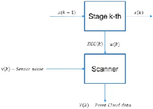
The model can be represented for a candidate sub-station as a function of the station KCCs and the incoming variations from previous stations. Figure 4 depicts the flow of information for a candidate station within a multi-stage manufacturing system.
Figure 4. Representation of a candidate station within a multi-stage manufacturing system
[image:5.595.221.373.545.653.2][𝐾𝐶𝐶̂ (𝑘), 𝑥̂(𝑘 − 1)] = 𝑓̂ (𝑌(𝑘) − 𝑌−1
0) (5)
The proposed model aims to approximate this function to enable the estimation of process parameters based on cloud-of-point data.
3.
PROPOSED MODEL
In the proposed model the function in Eqs. 4 or 5 is learned using supervised learning techniques in a regression-based setup. It is important to note that this function has no assumptions such as linearity of the system or independence between KCCs within the candidate substation. Given the 3D spatial correlation and dimension of cloud-of-point data, our proposed model PointDevNet leverages 3D convolutional neural networks (CNN) to estimate this function. The incoming part 𝑥̂(𝑘 − 1) is subject to variations also termed as part variations due to the previous manufacturing errors and the non-ideal nature of the part. 𝑥̂(𝑘 − 1) which is representative of the incoming part variation is obtained by considering the regression to be heteroskedastic and associating each observation with a variability factor 𝜎, that is estimated by considering a heteroskedastic loss function under Gaussian likelihood. The proposed model consists of various steps as described further.
3.1Data Generation
Data used for model training can be a collection of real data and simulated data obtained from finite element modelling simulators (first engineering principle models)27. The generated dataset consists of both cloud-of-point data and the KCCs
used to generate that cloud-of-points. A uniform random sample is drawn within the range of each process parameter (KCC). This sample is given as input to the FEM simulator which generates the deviations of each point within the points cloud.
3.2 Data Pre-processing – Voxelization of Cloud-of-point data
The application of 3D CNN 20 is enabled by voxelizing the cloud-of-points measurement data. Voxels are 3D grids of
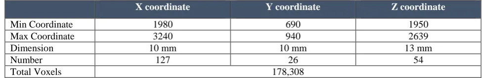
[image:6.595.50.544.463.542.2]arbitrary dimensions. The dimensions can be selected based on the required accuracy of predictions. Having smaller voxels provides great learnability but comes with larger computation cost. The selection will be dependent on the complexity of the manufacturing system and the required accuracy of process parameter prediction. Each point within the point cloud is mapped to a voxel-based on the point location. Each voxel can contain multiple points. Each point can have multiple components of deviations - ∆𝑥, ∆𝑦, and ∆𝑧. Each voxel is characterized by the maximum deviation considering all points that lie within the voxel. Table 1 summarizes the Voxelization for a window reinforcement panel. Each voxel has a dimension of 10 mm by 10 mm by 13 mm. This voxelized cloud-of-point is used for model training and predictions.
Table 1. Voxelization of Window Reinforcement Panel
3.3Model Architecture
Convolutional neural networks consist of multiple convolutions and fully connected layers to exploit the spatial correlations present in the input data and relate that to various classification or regression based outputs. The model consists of four 3D convolutional layers followed by two fully connected layers and an output layer. The hyperparameters and architecture are summarized in Figure 5. The initial convolutional layers help in feature extraction from cloud-of-point data, while the fully connected layers learn the relationships between features and process parameters. The hyper-parameters have been optimized using a grid search. All nodes within the network have ReLU activation units30 except the
output layer which consists of linear activation units since the output is a continuous real value.
X coordinate Y coordinate Z coordinate
Min Coordinate 1980 690 1950
Max Coordinate 3240 940 2639
Dimension 10 mm 10 mm 13 mm
Number 127 26 54
Figure 5. Model Architecture for PointDevNet
3.4Model Training
The equation used of model training is given below. Where [𝐾𝐶𝐶]𝑖 represents the actual value of the 𝑖 − 𝑡ℎ sample in the
training while 𝑓̂ (𝑌(𝑘) − 𝑌−1
0)𝑖 is the value estimated by the function. 𝜎𝑖represents the incoming magnitude of part
variation and measurement noise. The effect of measurement noise is homoscedastic since the same sensor is being used to measure each part:
𝐿(𝜃) = ∑ ‖[𝐾𝐶𝐶]𝑖−𝑓̂(𝑌(𝑘)−𝑌−1 0)𝑖‖ 2
2 𝜎𝑖2
𝑖 +
1 2log 𝜎𝑖
2 (6)
Adam31 is used to train and estimate the model parameters. Techniques such as dropout32 and batch normalization33 are
not effective as the model is used in a regression setup, not a classification setup. L2 norm regularization
(𝑅𝑒𝑔𝑢𝑙𝑎𝑟𝑖𝑧𝑖𝑛𝑔 𝑐𝑜𝑒𝑓𝑓𝑖𝑐𝑖𝑒𝑛𝑡 𝜆 = 0.01) is used in the fully connected layers to prevent overfitting. Max-pooling is not used since process parameter estimation does not permit translation invariance. Model training was done in python using distributed Tensorflow34 on a four node cluster with four Nvidia Quadro M2000 GPUs.
3.5Model Inference
The trained model can be used to estimate process parameters (KCCs) given cloud-of-point measurement data from optical metrology gauge after it has been voxelized. These KCC estimates from a manufacturing system can be analyzed as a time-series for 𝑛 𝑡𝑖𝑚𝑒 𝑠𝑡𝑒𝑝𝑠 to determine if there are any abnormalities such as mean shift, non-stationarity, heteroscedasticity or any other temporal pattern depending on the problem at hand. Lastly, optimized control actions can be performed within a closed loop. The model aims to eliminate the assumptions taken in state-of-the-art models such as linearity and independence of KCCs within a manufacturing system to enable effective root cause isolation and closed-loop control.
Figure 6. Framework for the application of the proposed model in a manufacturing system
Video 1: Framework and working of the proposed model, http://dx.doi.org/doi.number.goes.here
4.
CASE STUDY
4.1Experimental setup
For the validation of our model, we consider the deformation patterns that occur for sheet metal parts. Specifically, the considered sheet metal in this case study is a window-reinforcement panel for the subassembly of an automotive car door 5. The material is aluminium 5182 series and has a thickness of 2.2 mm.
patterns is essential in order to respond rapidly with corrective and control actions so as to address the process faults and guarantee the aforementioned functional and customer requirements. The model (PointDevNet) that is being proposed in this paper is able to identify single or multiple deformations patterns that are present in the sheet metal parts based on cloud-of-points data from the inspection robot.
In order to emulate different deformation patterns in a controlled way for the case study, a fixture design was considered that consisted of five clamps that can be moved in the y-direction (out-of-plane) to deform the part and introduce a specific pattern. Each of these clamps can be mapped to a different root cause. The sheet metal part in the fixture is then measured by the inspection robot and generates cloud-of-point data that represent the dimensions of the sheet metal part. Figure 7 below shows the CAD model for fixture design to emulate the deformation patterns. Figure 8 shows the five deformation patterns that occur due to five individual faults for the sheet metal part that is considered in this case study. Based on this cloud-of-point data, the variation of the deformation patterns is analysed in order to determine the root cause, which in this case are the y-positions of the five clamps. The performance of the proposed model PointDevNet is compared with that of the least squares linear model, the latter being the state-of-art technique for this purpose as proposed by Kavesh et al. 28.
The research would like to acknowledge that although this emulation is not representative of an actual assembly process it provides the required proof and insights to verify and validate the capabilities of the proposed model as well the limitations of the state-of-the-art model in terms of point selection and handling multiple interacting root causes. Future work entails application of the proposed model in an actual assembly process.
Data for model training is obtained using a FEM based simulator27. A triangular mesh with 8047 nodes was used to
[image:9.595.156.426.378.531.2]represent the window reinforcement panel as input to the Finite Element Method (FEM) based simulator. All clamps are varied in the y-direction to obtain deformation patterns. The variations of the clamps in the y-direction are the KCCs/root causes for this system. The model outputs the displacement (for six degrees-of-freedom: 𝑥, 𝑦, 𝑧, 𝛼, 𝛽, 𝛾) of the nodes for the deformed mesh. The node displacements in the y-direction are considered and this data is used for model training in a supervised framework. The point cloud data is post-processed to map the point cloud to the mesh nodes. Displacements in the y-direction are obtained by comparing this to the nominal mesh. These displacements are then used to validate if the model predictions correspond to the actual movement of the clamp in the fixture design.
Figure 7. Experimental setup: window-reinforcement panel and clamp location for deformation pattern emulation
[image:9.595.125.461.552.681.2]Training data generation is done considering a uniform sampling of the positioning of each clamp between ± 12 𝑚𝑚 in the y-direction. A total of 10,000 training samples are generated for model training and validation (8000: training, 2000: Testing). This data is used to train the proposed model, PointDevNet and state-of-the-art regression model. Each sample is generated with a different positioning for the five clamps within the given range. The hyper parameters for PointDevNet are given in Section 3. The results are compared with the state-of-the-art model for fault diagnosis which is a linear multiple regression model using least squares estimates. The proposed model, PointDevNet, is tested with state of the art model under different scenarios. The state of the art model uses five points as predictors given there are five KCCs that need to be predicted. Selecting less than five points will result in the system having many possible solutions for a given set of input points. Four different situations for the selection of these five points have been considered in the performed comparison study:
a) Optimal Point Selection (MR1): The nearest point where each of the five clamps touches the part are used as predictors b) Within 5 mm of the optimal point (MR2): The selected points lie within a 5 mm in-plane radius from the optimal point c) Within 10 mm of the optimal point (MR3): The selected points lie within a 10 mm in-plane radius from the optimal
point
d) Within 25 mm of the optimal point (MR4): The selected points lie within a 25 mm in-plane radius from the optimal point
The tests aim to compare the accuracy of prediction of the positioning of clamps (i.e. the root-causes in the considered case study) based on the cloud-of-point measurement data. Three different cases are considered below (for the state of the art regression model, all four situations stated above are considered for each case):
1. Single Root Cause (Case 1): Only one of the clamps can be moved at a time i.e. the part will have only one deformation pattern or root cause.
2. Multiple Root Cause (Case 2): More than one clamp can be moved simultaneously i.e. the part will have multiple deformation patterns or root causes.
3. Multiple Root Cause with Measurement Noise (Case 3): A random uniform number between ±0.1 𝑚𝑚 is added to each point within the point cloud to account for the measurement noise and other calibration errors for the clamp movement.
With this exercise, the paper aims to compare the performance of our proposed model, PointDevNet, with state-of-the-art regression model under these different scenarios. Prediction accuracy is compared in scenarios when only one root cause is present and when multiple root causes ar e present. Additionally, different point selection criteria are tested for the application of the state of the art model. Finally, the paper aims to learn the effect of measurement noise on the predictive ability for state of the art in comparison with the proposed model PointDevNet. Multiple runs for the sampling of training data and statistical tests are conducted to highlight the validity of the obtained results.
4.2Results and discussion
Single Root Cause (Case 1): Under conditions that only one fault is present both state-of-the-art and PointDevNet have similar accuracy metrics. The error of prediction for each deformation pattern (i.e. clamp displacement for the corresponding root cause) is less than 0.002 mm for the proposed model PointDevNet as well as the state of the art model for all four situations. There is no significant statistical difference in the accuracy of both models. Both models are able to estimate the root cause with high accuracy. It can thus be concluded that they have an equivalent performance for this purpose.
of prediction of the deformation pattern for each root cause (corresponding clamp movement) for the linear state-of-the-art model falls while the proposed model PointDevNet is able to estimate different root causes with higher accuracy.
Table 2. Mean absolute error comparison of PointDevNet with state of the art model considering multiple fault sources, all figures in mm (where there is a statistically significant difference, the minimum value is highlighted in bold)
Root Cause
PointDevNet MR1 MR2 MR4 MR4
Mean STD Mean STD Mean STD Mean STD Mean STD
Clamp 1 0.004 0.002 0.013 0.000 0.024 0.003 0.013 0.000 0.368 0.004
Clamp 2 0.010 0.003 0.025 0.000 0.096 0.001 0.052 0.001 0.227 0.004
Clamp 3 0.014 0.003 0.079 0.001 0.385 0.005 0.645 0.005 1.021 0.009
Clamp 4 0.017 0.002 0.037 0.001 0.073 0.001 0.207 0.002 1.365 0.017
Clamp 5 0.006 0.003 0.070 0.001 0.071 0.001 1.493 0.020 2.988 0.035
Multiple Root Cause and Measurement Noise (Case 3): Measurement noise and fixture repeatability noise can be present in a system, typically with a magnitude up to ±0.1 𝑚𝑚 for the system in the considered case study. As done for Case 2, the Mean Absolute Error (MAE) is used as the metric to evaluate model performance as opposed to Root Mean Square Error (RMSE) because in context to KCC estimation all errors should be penalized equally and MAE values are easily interpretable as an average of absolute error values. The mean and standard deviation (STD) of the MAE for nine runs for each root cause is given in Table 3. Measurement error leads to a further drop in accuracy for the state-of-the-art model while there is no major difference in model accuracy for PointDevNet. As established in the literature, overfitting 37 is a
common problem for Convolutional neural networks and the addition of artificial noise is a technique used to prevent overfitting. Therefore, the presence of measurement noise aids regularization 38 and prevents overfitting. As seen from
results for clamps 2, 4 and 5, PointDevNet has a slightly higher accuracy of prediction in Case 3 compared to Case 2.
Conducting ANOVA test on MAE for each root cause shows a significant difference between all four groups (p-value > 99.99%). Post-hoc analysis is done using a Tukey-HSD test at 95% significance to determine which pairs of mean have a significant difference. Except MR1 and MR3 for clamp 1 and MR1 and MR2 for clamp 5, all other pairs are statically significant at 95% significance level. Figure 9 compares the mean MAE for Case 3 across all root causes. The results show that the accuracy of state of the art model falls even more while the proposed PointDevNet model is robust to measurement noise due to inherent noise filtration of convolutional functions present within the PointDevNet model. It can be concluded from the presented results that when there are multiple root causes and measurement noise, the proposed PointDevNet model outperforms the state-of-the-art model. Additionally, for the application of the state-of-the-art model, point-selection is critical. As shown in Cases 2 and 3, there is a significant drop in accuracy when the point selection is suboptimal while for the application of our proposed model point-selection need not be done. Although it is necessary to acknowledge the limitation of the proposed PointDevNet model in that it is only applicable to cloud-of-point data, or it would require an impractically large amount of point-based measurement data.
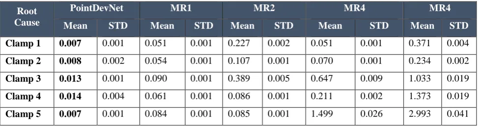
Table 3. Mean absolute error comparison of PointDevNet with state of the art model considering multiple fault sources and measurement noise, all figures in mm (the minimum value is highlighted in bold)
Root Cause
PointDevNet MR1 MR2 MR4 MR4
Mean STD Mean STD Mean STD Mean STD Mean STD
Clamp 1 0.007 0.001 0.051 0.001 0.227 0.002 0.051 0.001 0.371 0.004
Clamp 2 0.008 0.002 0.054 0.001 0.107 0.001 0.070 0.001 0.234 0.002
Clamp 3 0.013 0.001 0.090 0.001 0.389 0.005 0.647 0.009 1.033 0.019
Clamp 4 0.014 0.004 0.061 0.001 0.086 0.001 0.211 0.002 1.373 0.019
[image:11.595.55.543.557.686.2]Figure 9. Comparison for multiple root-cause and measurement noise (Case 3)
5.
CONCLUSIONS
This paper proposes a new model, PointDevNet, for process parameter (KCC) variation estimation to aid root cause analysis and closed-loop control for an assembly process considering parts to be compliant using cloud-of-point measurement data. The model performs better in terms of handling interactions of multiple fault sources (KCC variations) than state-of-the-art models that use single point measurement data. The model is also robust to measurement noise which is a major problem in measurement systems. Additionally, point selection is critical when it comes to the application of state of the art models but our model does not have to deal with point selection. Different point selection techniques have not been evaluated in this paper though this remains a focus for future work. It is worth noting that as the root cause problem is scaled up to more complex assemblies such as joining using riveting or laser welding consisting of significantly higher interactions and process parameters, the proposed model can potentially perform better given the inherent ability of deep neural networks to model complex non-linear relationships as opposed to linear state-of-the-art models. Future work should also include using the proposed model, PointDevNet, for quality control in other manufacturing systems, beyond assembly, for example, to characterise dimensional variations that occur in multi-stage sheet metal press line39.
Given the model is trained on a representative sample it is able to diagnose systems with much higher dimensionality (number of root causes) having a higher degree of interactions. In scientific terms, the results of this paper demonstrates
(1) application of 3D convolutional neural networks to build a model capable of diagnosing assembly systems considering interactions between multiple root causes and measurement noise without the need for point selection; and (2) a model capable of analyzing high dimensional cloud-of-point data from the white-light stereovision system (Multi-wave Light Technology). Industrial Contribution may be seen as the integration of this model within a manufacturing system that can enable closed-loop control which reduces machine downtime and increases productivity, while also enabling efficient predictive maintenance and continuous improvement of product quality.
Future work entails the use of the proposed model for sheet metal assemblies where abnormal variations in assembly process parameters such as fixturing and tooling lead to deformation patterns in the final assemblies. Trained on a representative sample of the assembly behaviour under different process parameter variations, PointDevNet can isolate process parameter variations leading to abnormal assembly behaviour. Given the inherent complexity present within assembly systems4041, CNNs are well-suited for diagnosing such complex systems given their ability to complex
non-linear functions.
ACKNOWLEDGEMENTS
REFERENCES
[1] Huang, W., Lin, J., Bezdecny, M., Kong, Z. and Ceglarek, D., “Stream-of-Variation Modeling—Part I: A Generic Three-Dimensional Variation Model for Rigid-Body Assembly in Single Station Assembly Processes,” J. Manuf. Sci. Eng. 129(4), 821 (2007).
[2] Ceglarek, D. and Shi, J., “Dimensional variation reduction for automotive body assembly,” Manuf. Rev. Vol. 8, 139–154 (1995).
[3] Liu, Y. G. and Hu, S. J., “Assembly Fixture Fault Diagnosis Using Designated Component Analysis,” J. Manuf. Sci. Eng. 127(2), 358 (2005).
[4] Apley, D. W. and Shi, J., “Diagnosis of Multiple Fixture Faults in Panel Assembly,” J. Manuf. Sci. Eng. 120(4), 793 (2008).
[5] Yu, K. G., Jin, S. and Lai, X. M., “Fixture variation diagnosis of compliant assembly using sensitivity matrix,” J. Shanghai Jiaotong Univ. (2009).
[6] Liu, Y., Jin, S., Lin, Z., Zheng, C. and Yu, K., “Optimal sensor placement for fixture fault diagnosis using Bayesian network,” Assem. Autom. (2011).
[7] Camelio, J. A., Hu, S. J. and Yim, H., “Sensor Placement for Effective Diagnosis of Multiple Faults in Fixturing of Compliant Parts,” J. Manuf. Sci. Eng. (2005).
[8] Carlson, J. S. and Söderberg, R., “Assembly root cause analysis: A way to reduce dimensional variation in assembled products,” Int. J. Flex. Manuf. Syst. (2003).
[9] Jin, S., Liu, Y. and Lin, Z., “A Bayesian network approach for fixture fault diagnosis in launch of the assembly process,” Int. J. Prod. Res. 50(23), 6655–6666 (2012).
[10] Ceglarek, D. and Shi, J., “Fixture Failure Diagnosis for Autobody Assembly Using Pattern Recognition,” J. Eng. Ind. 118(1), 55 (1996).
[11] Ceglarek, D. and Shi, J., “Fixture Failure Diagnosis for Sheet Metal Assembly with Consideration of Measurement Noise,” J. Manuf. Sci. Eng. 121(4), 771 (1999).
[12] Shiu, B. W., Ceglarek and Shi, H., “Multi-stations sheet metal assembly modeling and diagnostics” (1996). [13] Ceglarek, D., Shi, J. and Wu, S. M., “A Knowledge-Based Diagnostic Approach for the Launch of the Auto-Body
Assembly Process,” J. Eng. Ind. 116(4), 491 (1994).
[14] Huang, W., Lin, J., Kong, Z. and Ceglarek, D., “Stream-of-Variation (SOVA) Modeling II: A Generic 3D Variation Model for Rigid Body Assembly in Multi Station Assembly Processes,” Manuf. Eng. Text. Eng. 2006, 323–333, ASME (2006).
[15] Ding, Y., Ceglarek, D. and Shi, J., “Fault Diagnosis of Multistage Manufacturing Processes by Using State Space Approach,” J. Manuf. Sci. Eng. 124(2), 313 (2002).
[16] Kong, Z., Ceglarek, D. and Huang, W., “Multiple Fault Diagnosis Method in Multistation Assembly Processes Using Orthogonal Diagonalization Analysis,” J. Manuf. Sci. Eng. 130(1), 011014 (2008).
[17] Ding, Y., Gupta, A. and Apley, D. W., “Singularity Issues in Fixture Fault Diagnosis for Multi-Station Assembly Processes,” J. Manuf. Sci. Eng. 126(1), 200 (2004).
[18] Franciosa P., Sun T., Ceglarek D., Gerbino S., L. A., “Multi-Wave Light Technology to Enable Closed-Loop In-Process Quality Control with Application to Remote Laser Welding of Battery Systems,” SPIE proceedings- Opt. Metrol. Int. Congr. Cent. Munich, Ger. 24 - 27 June 2019 (2019).
[19] Qi, C. R., Su, H., Mo, K., Guibas, L. J., Charles, R. Q., Su, H., Kaichun, M., Guibas, L. J., Qi, C. R., Su, H., Mo, K. and Guibas, L. J., “Pointnet: Deep learning on point sets for 3d classification and segmentation,” Proc. Comput. Vis. Pattern Recognit. (CVPR), IEEE 1(2), 4 (2017).
[20] Maturana, D. and Scherer, S., “VoxNet: A 3D Convolutional Neural Network for real-time object recognition,” IEEE Int. Conf. Intell. Robot. Syst., 922–928, IEEE (2015).
[21] Mitchell, T. M., “Machine learning and data mining,” Commun. ACM 42(11), 30–36 (1999).
[22] Leibig, C., Allken, V., Ayhan, M. S., Berens, P. and Wahl, S., “Leveraging uncertainty information from deep neural networks for disease detection,” Sci. Rep. 7(1), 17816 (2017).
[23] Qi, C. R., Yi, L., Su, H. and Guibas, L. J., “PointNet++: Deep Hierarchical Feature Learning on Point Sets in a Metric Space” (2017).
[24] Monostori, L., Markus, A., Van Brussel, H. and Westkämpfer, E., “Machine Learning Approaches to Manufacturing,” CIRP Ann. 45(2), 675–712 (1996).
[26] Pham, D. T. and Afify, A. A., “Machine-learning techniques and their applications in manufacturing,” Proc. Inst. Mech. Eng. Part B J. Eng. Manuf. 219(5), 395–412 (2005).
[27] P. Franciosa, Ceglarek, D., “Variation Response Method (VRM) Simulation toolkit,” 3.0 (2018).
[28] Bastani, K., Barazandeh, B. and Kong, Z., “Fault Diagnosis in Multistation Assembly Systems Using Spatially Correlated Bayesian Learning Algorithm,” J. Manuf. Sci. Eng. 140(3), 031003 (2017).
[29] Jin, J. and Shi, J., “State Space Modeling of Sheet Metal Assembly for Dimensional Control,” J. Manuf. Sci. Eng.
121(4), 756 (1999).
[30] Krizhevsky, A., Sutskever, I. and Hinton, G. E., “ImageNet Classification with Deep Convolutional Neural Networks,” 1097–1105 (2012).
[31] Kingma, D. P. and Ba, J., “Adam: A Method for Stochastic Optimization” (2014).
[32] Srivastava, N., Hinton, G., Krizhevsky, A., Salakhutdinov, R., Sutskever, I. and Salakhutdinov, R., “Dropout: A Simple Way to Prevent Neural Networks from Overfitting,” Dropout A Simple W. to Prev. Neural Networks from Overfitting 15, 1929–1958 (2014).
[33] Ioffe, S. and Szegedy, C., “Batch Normalization: Accelerating Deep Network Training by Reducing Internal Covariate Shift” (2015).
[34] GoogleResearch., “TensorFlow: Large-scale machine learning on heterogeneous systems,” Google Res. (2015). [35] Yang, J.-H. and Yang, M.-S., “A control chart pattern recognition system using a statistical correlation coefficient
method,” Comput. Ind. Eng. 48(2), 205–221 (2005).
[36] Hirsch, J., “Recent development in aluminium for automotive applications,” Trans. Nonferrous Met. Soc. China
24(7), 1995–2002 (2014).
[37] Hawkins, D. M., “The Problem of Overfitting” (2003).
[38] Poggio, T., Torre, V. and Koch, C., “Computational vision and regularization theory,” Readings Comput. Vis., 638–643 (1987).
[39] Glorieux, E., Franciosa, P. and Ceglarek, D., “End-effector design optimisation and multi-robot motion planning for handling compliant parts,” Struct. Multidiscip. Optim. 57(3), 1377–1390 (2018).
[40] Franciosa, P., Palit, A., Vitolo, F. and Ceglarek, D., “Rapid Response Diagnosis of Multi-stage Assembly Process with Compliant non-ideal Parts using Self-evolving Measurement System,” Procedia CIRP 60, 38–43 (2017). [41] Rong, Q., Shi, J. and Ceglarek, D., “Adjusted Least Squares Approach for Diagnosis of Ill-Conditioned Compliant