A framework for quantification of human structure interaction in vertical direction

Original citation:

Ahmadi, Ehsan, Caprani, Colin, Živanović, Stana, Evans, Neil D. and Heidarpour, Amin (2018) A framework for quantification of human-structure interaction in vertical direction. Journal of Sound and Vibration, 432 . pp. 351-372. doi:10.1016/j.jsv.2018.06.054

Permanent WRAP URL:

http://wrap.warwick.ac.uk/103971

Copyright and reuse:

The Warwick Research Archive Portal (WRAP) makes this work by researchers of the University of Warwick available open access under the following conditions. Copyright © and all moral rights to the version of the paper presented here belong to the individual author(s) and/or other copyright owners. To the extent reasonable and practicable the material made available in WRAP has been checked for eligibility before being made available.

Copies of full items can be used for personal research or study, educational, or not-for-profit purposes without prior permission or charge. Provided that the authors, title and full bibliographic details are credited, a hyperlink and/or URL is given for the original metadata page and the content is not changed in any way.

Publisher’s statement:

© 2018, Elsevier. Licensed under the Creative Commons Attribution-NonCommercial-NoDerivatives 4.0 International http://creativecommons.org/licenses/by-nc-nd/4.0/

A note on versions:

The version presented here may differ from the published version or, version of record, if you wish to cite this item you are advised to consult the publisher’s version. Please see the ‘permanent WRAP url’ above for details on accessing the published version and note that access may require a subscription.

A Framework for Quantification of Human-Structure Interaction

in Vertical Direction

Ehsan Ahmadi1_{, Colin Caprani}1_{*, Stana Živanović}2_{, Neil Evans}2_{, Amin Heidarpour}1

3 

1 _{Dept. of Civil Engineering, Monash University, Australia}

4 

2 _{School of Engineering, University of Warwick, UK}

5 

* Corresponding Author

6 

7 

8 

9 

10 

11 

Abstract

12 

In lightweight structures, there is increasing evidence of the existence of interaction between

13 

pedestrians and structures, now commonly termed pedestrian-structure interaction. The

14 

presence of a walker can alter the dynamic characteristics of the human-structure system

15 

compared with those inherent to the empty structure. Conversely, the response of the structure

16 

can influence human behaviour and hence alter the applied loading. In the past, most effort on

17 

determining the imparted footfall-induced vertical forces to the walking surface has been

18 

conducted using rigid, non-flexible surfaces such as treadmills. However, should the walking

19 

surface be vibrating, the characteristics of human walking could change to maximize comfort.

20 

Knowledge of pedestrian-structure interaction effects is currently limited, and it is often quoted

21 

as a reason for our inability to predict vibration response accurately. This work aims to quantify

22 

the magnitude of human-structure interaction through a experimental-numerical programme

23 

on a full-scale lively footbridge. An insole pressure measurement system was used to measure

24 

the human-imparted force on both rigid and lively surfaces. Test subjects, walking at different

25 

pacing frequencies, took part in the test programme to infer the existence of the two forms of

26 

human-structure interaction. Parametric statistical hypothesis testing provides evidence on the

27 

existence of human-structure interaction. In addition, a non-parametric test (Monte Carlo

28 

simulation) is employed to quantify the effects of numerical model error on the identified

29 

human-structure interaction forms. It is concluded that human-structure interaction is an

important phenomenon that should be considered in the design and assessment of

vibration-31 

sensitive structures.

32 

33 

Keywords

34 

Human-structure interaction; footbridge vibration; experiment; in-sole sensors

35 

36 

1. Introduction

37 

Many newly built structures have light weight, low damping, and low stiffness, and they may

38 

not satisfy vibration serviceability criteria when occupied and dynamically excited by humans

39 

[1]. Observed problems have been caused typically by human occupants performing normal

40 

activities such as walking, running, jumping, bouncing/bobbing, and dancing. Vibration

41 

beyond the human comfort range will influence human comfort and so is a key consideration

42 

for designers. Human presence can affect the dynamic characteristics of the coupled

human-43 

structure system during motion, named here as Human-to-Structure Interaction (H2SI). On the

44 

other hand, the vibrating structure may change the human activity force pattern, and this

45 

potential phenomenon is named here as a Structure-to-Human Interaction (S2HI) (Figure 1).

46 

These postulated mutual effects between human and structure are collectively referred to as

47 

human-structure interaction (HSI). Since for this work we consider only single human loading

48 

situations, we do not consider human-to-human interaction which can take place in crowds.

49 

The H2SI and S2HI effects are usually considered mutually exclusive [2], meaning that HSI is

50 

often modelled through a change in the dynamic properties of the system only or a change in

51 

walking force only. In this study, they are assumed to be mutually independent, isolated and

52 

examined individually using a novel experimental-numerical programme while both types

53 

occur simultaneously.

54 

The focus of this study is on human walking and the resulting vibration. To assess the vibration

56 

response of structures susceptible to human walking, accurate estimation of human force,

57 

dynamic characteristics of the structure, and human-structure interaction are required

58 

(Figure 1). As a novel aspect of this work, human walking force was measured using TekScan

59 

F-scan in-shoe plantar pressure sensors intended for medical applications. The plantar pressure

60 

force gives a reliable measurement of the vertical walking force [3], [4]. Further, the mass,

61 

damping, and stiffness of the structure were obtained using system identification methods. The

62 

most challenging part of the study of human-structure interaction is to identify and quantify the

63 

postulated forms of HSI separately. This study proposes an experimental framework to address

64 

this challenge. It relies on acquiring sufficiently accurate measurements of the human force,

65 

structure dynamics, and comparison of data recorded on rigid and flexible surfaces. The two

66 

postulated forms of HSI will be described in more detail in the next two sections.

67 

68 

Figure 1 Interactions between humans and the structure in the human-structure system are collectively called

69 

Human-Structure Interaction (HSI), but are considered separately here as Human-to-Structure Interaction

70 

(H2SI) and Structure-to-Human Interaction (S2HI).

71 

72 

The human body is a sensitive vibration receiver characterized by an innate ability to adapt

73 

quickly to almost any type and level of vibration which normally occurs in nature [5]. This

74 

effective self-adapting mechanism triggers pedestrians to change their walking behaviour [6].

75 

In turn, it leads to walking force patterns that can be different to those measured on

non-76 

vibrating rigid surfaces [7].

There have been numerous attempts to measure or model pedestrian-induced forces, referred

79 

to as ground reaction forces (GRFs); see for example [8], [9], [10], [11], [12], [13], [14]. Past

80 

GRF measurement facilities typically comprised equipment for direct force measurements,

81 

such as a force plate [15], or an instrumented treadmill usually mounted on rigid laboratory

82 

floors ([16], [17], [18]). However, GRFs could differ when walking on vibrating surface. For

83 

example, Ohlsson [19] found that the vertical force measured on a flexible timber floor is

84 

different from that measured on a rigid base. Pavic et al. [20] pointed out that the force induced

85 

by jumping on a flexible concrete beam was lower than that on a force plate. Van Nimmen et

86 

al. [21] and Bocian et al. [22] indirectly reconstructed vertical walking force on bridge surfaces

87 

from inertial motion tracking and a single point inertial measurement respectively. To the

88 

authors’ knowledge, Dang and Zivanovic [23] is the only experimental work on direct

89 

measurement of walking GRFs on lively structures in the vertical direction. The results showed

90 

a drop in the first dynamic load factor of the walking force due to the bridge vibration at the

91 

resonance. However, test subjects walked on-the-spot on a treadmill for this study.

92 

93 

Humans add mass, stiffness, and damping to the coupled human-structure system. The

94 

influence of passive humans on the dynamic properties of the structure they occupy (i.e. modal

95 

mass, damping, and stiffness) have been well-documented in the literature [24], [2], [25], [26].

96 

For example, Ohlsson [19] found that a walking pedestrian can increase the HSI system’s

97 

frequency and damping, while Willford [27] also reported a change in the system’s damping

98 

due to moving crowd in the vertical direction. Zivanovic et al. [28] and Van Nimmen et al. [29]

99 

identified modal properties of the HSI system and showed that the presence of humans on the

100 

structure, either in standing or walking form, will increase the damping of the system compared

101 

to the empty structure. Zivanovic et al. [30] revealed that crowd effects can be also modelled

102 

as an increase in the damping of the system, in some cases more than two times greater than

the damping ratio for the empty bridge, and Caprani et al. [31] did so to account for crowd

104 

damping effects. Kasperski [32] also concluded that a walking pedestrian can induce additional

105 

damping by using discrete Fourier transform of the acceleration time history response of the

106 

bridge. However, these existing effects are not incorporated into design codes and guidelines

107 

such as OHBDC [33], U.K. National Annex to Eurocode 1 (British Standards Institution 2008)

108 

[34], ISO-10137 [35], Eurocode 5 [36], Setra [37], and HIVOSS [38] as they model humans as

109 

a moving force only. Interestingly, the U.K. National Annex to Eurocode 1 does acknowledge

110 

that H2SI effects exist, but does not offer guidance on their inclusion, underlining the need to

111 

quantify the H2SI effect on vibration.

112 

113 

The review above has shown that quantification of human-structure interaction is a crucial part

114 

of vibration response estimation and that there is some evidence of the two postulated forms of

115 

HSI in the literature. However, these HSI forms are not fully experimentally quantified, which

116 

is an essential step towards the development of design/assessment guidelines that can consider

117 

HSI. This work experimentally investigates the existence of the two postulated HSI forms by

118 

isolating their influence on the vibration response. To this end, a novel experimental-numerical

119 

programme is adopted. The human-imparted forces to both flexible (i.e. footbridge) and rigid

120 

surfaces are measured. These are then used to simulate the vibration response. The simulated

121 

vibration response from walking force measured on the rigid surface represents state-of-the-art

122 

practice. The vibration response of the footbridge is also directly measured. Comparison of

123 

dynamic load factors of the forces on the bridge surface with those of rigid surface should

124 

reveal any walking pattern change due to HSI (S2HI). Another comparison for simulated

125 

vibration responses due to the rigid and bridge surface walking forces discloses the effect of

126 

S2HI on the vibration response. Comparing the simulated bridge vibration response and the

127 

system dynamic characteristics (H2SI). A parametric statistical hypothesis test is then used to

129 

show the generality of the results for a large number of walking trial scenarios. Finally, a

non-130 

parametric test (Monte Carlo simulation) is conducted to determine the influence of model

131 

errors on the two postulated forms of HSI. This experimental-numerical approach is next

132 

described in detail.

133 

134 

2. Experimental Procedure

135 

2.1 Experimental-numerical programme

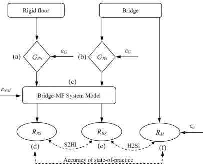
136 

Figure 2 schematically illustrates the experimental-numerical programme design to investigate

137 

HSI. Two types of measurement are taken: (1) GRFs from walking on a rigid surface (RS), GRS

138 

(part (a) in Figure 2); (2) GRFs from walking on a vibrating bridge surface (BS), GBS (part (b)),

139 

while the vibration response of the bridge, RM (part (f)), is concurrently measured. Subsequent

140 

to these physical measurements, vibration responses to the measured RS and BS GRFs are

141 

simulated using a system model (part (c)), namely a modal model of the bridge and a moving

142 

force (MF) model of the pedestrian. These were denoted RRS (part (d)), and RBS (part (e)),

143 

respectively.

144 

146 

Figure 2 A schematic overview of the experimental-numerical programme, including an assessment of the

147 

accuracy of typical current practice using a moving force approach.

148 

149 

In this study, a difference between the vibration responses RRS (part (d)) and RBS (part (e)) of

150 

the analytical model is considered as evidence of the influence of the vibrating bridge surface

151 

on the walker-induced force (S2HI) (part (a) versus part (b)). Going a step farther, comparing

152 

the simulated vibration response, RBS , to those measured from the bridge, RM , yields the

153 

accuracy of the coupled bridge-MF system model (part (c)) itself. Here, there are two potential

154 

errors to the system model: (1) the accuracy of the bridge model, and (2) the accuracy of MF

155 

model due to H2SI. A reliable system identification method and using amplitude-dependent

156 

frequency and damping of the bridge can significantly increase the accuracy of the bridge

157 

model and reduce the first source of error in the system model to a very small amount.

158 

Consequently, any difference between RBS and RM is because the MF model is unable to insert

159 

human effects into the numerical model, H2SI. Further, comparison of RRS and RM implies the

accuracy of state-of-the-art design practice as the MF model and rigid surface force are used to

161 

estimate the actual bridge response RM.

162 

163 

The influence of errors in various measurements, is also considered. The system numerical

164 

model error, NM, and measurement errors, G and a will be discussed later. Monte Carlo

165 

simulations are performed to evaluate the influence of these errors (which are difficult to

166 

measure) on the HSI quantifications.

167 

168 

2.2 Walking trials

169 

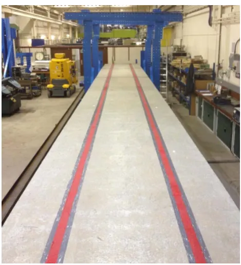
All tests were carried out on the Warwick Footbridge – a steel-concrete composite laboratory

170 

footbridge at the University of Warwick, UK, shown in Figure 3. The bridge is a unique

171 

laboratory structure purpose-built with a natural frequency in the vertical direction that can be

172 

matched by pacing rate, making it an ideal facility for studying HSI. The simply-supported

173 

span length of the bridge is adjustable, but was kept constant throughout the tests at 16.2 m.

174 

The bridge is 2 m wide, with a clear walkway track down the centre. The bridge mass is

175 

approximately 16500 kg, and the modal mass of the first bending mode is 7614 kg with natural

176 

frequency of about 2.43 Hz [39]. As a unique facility, it has already been used considerably for

177 

the study of human-induced vibration [23].

178 

180 

Figure 3 The Warwick footbridge.

181 

182 

The tests comprised of walking at 2.4 Hz to excite the resonance by the first forcing harmonic,

183 

walking at 1.2 Hz to excite the resonance by the second harmonic, and walking at 2.1 Hz to

184 

expose the test subject to the beating vibration response. 2.4 Hz covers upper bound of normal

185 

pacing frequency range of a pedestrian (1.6-2.4 Hz). In this paper, the pacing-to-bridge

186 

frequency ratio ( = fp/fb) is used, and so β {0.5, 0.87, 1.0}.

187 

188 

Five test subjects (4 male, 1 female), weighing from 543 N to 1117 N participated in the

189 

experiments. The test subject-to-bridge mass ratio, m = mp/mbranged from 0.33-0.7% and it

190 

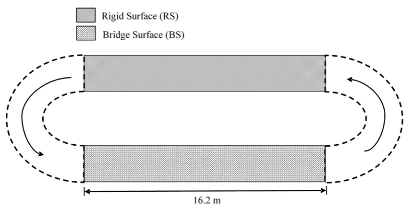
will be used later to discuss the results for each test subject. For each trial, test subjects walked

191 

a circuit including a rigid surface (RS) and bridge surface (BS) as shown in Figure 4. On both

192 

surfaces, the walking length was the same (16.2 m). After a sound signal, test subjects started

193 

walking. A metronome was used during each trial so that test subjects targeted the desired

194 

pacing frequency. Each walking trial was repeated until five successful trials were recorded. It

195 

should be stated that all trials were carried out in accordance with The Code of Ethics of the

198 

199 

200 

Figure 4 Schematic plan of the walking trials path.

201 

202 

2.3 Data acquisition

203 

To record input forces and output accelerations data, a test set-up was designed as shown in

204 

Figure 5. The bridge vibration was measured using two Honeywell QA750 accelerometers,

205 

placed at mid-span and quarter-span points. The accelerometer signals were recorded using

206 

Quattro data acquisition (DAQ) unit by Data Physics (see Figure 5). The TekScan equipment

207 

was used for collecting the GRFs of the rigid and bridge surfaces throughout the walking trials.

208 

A TekScan trigger transmitter and two TekScan trigger receivers were used to synchronize

209 

recordings remotely. One trigger receiver was connected to the data recorder of the TekScan

210 

system, and the other one was attached to the Quattro DAQ. Note that unusually, the trigger

211 

was not used to trigger recording, rather its voltage output was recorded to identify the time

212 

window when the test subject was occupying the bridge. Thus, when the test subject was

213 

visually observed to be at the end of the footbridge a further trigger signal was given, changing

214 

the trigger output voltage, though data continued to be collected (e.g. free-vibration). Figure 6

215 

shows a typical trigger voltage signal for the test subject of μm = 0.6 % and trial No. 5 with

frequency ratio of 1. This specific test subject, trial, and frequency ratio will be used as a

217 

running example through the paper.

218 

219 

220 

Figure 5 Test set-up for data acquisition.

221 

222 

0 5 10 15 20

2.4 2.42 2.44 2.46 2.48 2.5 2.52

t (s)

Vo

lt

a

g

e Time on the bridge

Time off the bridge

223 

Figure 6 Voltage signal for time on and off the bridge for the example test subject, μm = 0.6 % and trial No. 5

224 

with frequency ratio of 1.

225 

3. Experimental Results

227 

3.1 Footbridge frequency and damping

228 

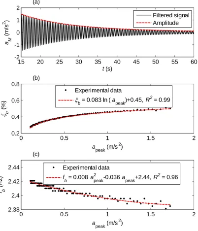
Free decay vibration measurements were made to investigate dynamic characteristics of the

229 

footbridge. It was found that the bridge frequency, fb, and damping, ξb, are amplitude-dependent.

230 

To determine the bridge damping, an exponential decay curve is fitted (using least-squares) to

231 

a moving window of five peaks (Figure 7a). It was found that the damping ratio increases with

232 

an increase in the vibration amplitude, ap, as shown in Figure 7b. This is a common feature of

233 

real structures because there are more sources and increased energy dissipation at higher

234 

vibration amplitudes. Nevertheless, the maximum damping ratio of about 0.5% is still quite

235 

low, ensuring lively behaviour. The natural frequency was found to decrease slightly with an

236 

increase in the vibration amplitude (Figure 7c). This is also typical behaviour in civil

237 

engineering structures. Finally, data points were fitted to model the relationship between

238 

damping and vibration amplitude, as well as frequency and vibration amplitude (Figures 7b

239 

and 7c). These relationships are used in the numerical simulations.

240 

15 20 25 30 35 40 45 50 55 60 -2

-1 0 1 2

t (s) a M

(

m

/s

2 )

(a)

Filtered signal Amplitude

0 0.5 1 1.5 2

0.2 0.4 0.6 0.8

a

peak (m/s

2

)

 b

(%)

(b)

Experimental data



b = 0.083 ln (apeak)+0.45, R

2 _{= 0.99}

0 0.5 1 1.5 2

2.38 2.4 2.42 2.44

a

peak (m/s

2

) f b

(H

z

)

(c)

Experimental data

f

b = 0.008 apeak

2

-0.036 a

peak+2.44, R

2

= 0.96

242 

Figure 7 (a) free decay vibration time history and its amplitude for the bridge (a low-pass 4th order Butterworth

243 

filter with cut-off frequency, 10 Hz, was used); (b) amplitude-dependent bridge damping results and model (c)

244 

amplitude-dependent bridge frequency results and model.

245 

246 

3.2 Measured vibration responses

247 

The mid-span acceleration response of the bridge to a walking trial, in which a test subject

248 

walked at 2.4 Hz (hereafter referred to as the exemplary test subject and trial), is illustrated in

249 

Figure 8a. Noise in the measured signal was removed using a low-pass 4th order Butterworth

filter with cut-off frequency of 10 Hz. The cut-off frequency of 10 Hz is more than four times

251 

the bridge fundamental frequency and so the results will not be influenced by the filter roll-off.

252 

The corresponding power spectrum density (PSD) of the acceleration signal, shown in Figure

253 

8b, reveals that most of the response energy is concentrated at the first vibration mode of the

254 

bridge.

255 

256 

257 

Figure 8 (a) bridge mid-span acceleration response (b) its corresponding power spectral density (PSD) for the

258 

exemplary test subject (trial of Figure 6).

259 

260 

The maximum response for each acceleration signal is selected as the response metric. Table 1

261 

summarizes the maximum acceleration response, amax, for each test subject, pacing frequency,

262 

and trial. The maximum accelerations from Table 1 can be compared with the limits in the

263 

0 20 40 60 80 100 120

-2 -1 0 1 2

a M

(m

/s

2 )

t (s) (a)

Original signal Filtered signal

0 2 4 6 8 10

10-5 100

PS

D (

m

2 /s 4 /H

z

)

Setra guideline [37], shown in Table 2. In many cases, the footbridge provides either “minimum”

264 

or “unacceptable vibration” comfort level to the test subject, demonstrating the liveliness of

265 

the structure.

266 

267 

Table 1. Maximum measured acceleration response (amax, m/s2).

268 

Test Subject

Mass Ratio, m (%)

Frequency Ratio, 

Trial No.

Mean 1 2 3 4 5

1 0.33

0.50 0.22 0.22 0.21 0.22 0.25 0.22

0.87 0.17 0.21 0.20 0.15 0.19 0.18

1.00 1.32 1.40 1.28 1.24 1.33 _1.31

2 0.40

0.50 0.19 0.17 0.17 0.18 0.20 _0.18

0.87 0.19 0.24 0.17 0.16 0.20 0.19

1.00 1.26 1.43 1.32 1.28 1.26 1.31

3 0.50

0.50 0.16 0.25 0.15 0.20 0.18 _0.19

0.87 0.35 0.20 0.22 0.22 0.22 _0.24

1.00 1.33 1.05 1.43 1.32 1.43 1.31

4 0.60

0.50 0.25 0.23 0.25 0.37 0.30 0.28

0.87 0.21 0.28 0.28 0.27 0.24 _0.26

1.00 1.34 1.83 1.82 1.84 1.87 _1.74

5 0.70

0.50 0.49 0.53 0.46 0.62 0.57 0.53

0.87 0.29 0.35 0.54 0.28 0.37 0.37

1.00 2.48 2.38 2.63 2.50 2.53 _2.51

269 

Table 2. Comfort levels and acceleration ranges (from [7]).

270 

Comfort Level Degree of comfort Vertical acceleration limits (m/s2₎

CL 1 Maximum < 0.5

CL 2 Medium 0.5 – 1.0

CL 3 Minimum 1.0 – 2.5

CL 4 Unacceptable vibration > 2.5

271 

3.3 GRFs signal acquisition and processing

272 

To measure the GRFs on both the rigid and flexible surfaces during walking, a novel

273 

experimental approach was employed. TekScan F-Scan in-shoe plantar pressure sensors

274 

developed for medical applications were used [3], [40], [41]. The measured pressure profiles

were integrated to determine force time histories for each foot allowing detailed gait analysis.

276 

TekScan F-scan in-shoe sensors, pressure distribution, and bridge surface force signals, GBS,

277 

of left and right feet for the exemplary test subject are shown in Figure 9.

278 

279 

The sensors are made up of 960 individual pressure sensing capacitor cells, which are referred

280 

to as sensels. The sensels are arranged in rows and columns on each sensor. The 8-bit output

281 

of each sensel is divided into 28 _{= 256 increments, and displayed as a value (Raw Sum), in the}

282 

range of 0 to 255 by the F-scan software. If all sensels reach a raw count of 255, the

283 

corresponding pressure is called saturation pressure. Although raw sum display shows relative

284 

force differences on the sensor, this data is more meaningful if the force is calibrated to give

285 

engineering measurement units. Obviously, proper calibration of the sensors is critical to

286 

obtaining accurate force readings. When a test subject walks, there must be sufficient raw

287 

output generated from the sensor so the calibration is accurate. It is also necessary to zero the

288 

sensor output. Indeed, when one foot is supporting the body weight during walking, the other

289 

foot is up in the air and its force should be zero. However, because the foot sensors are

pre-290 

tensioned to the sole of the foot by shoe-lacing, the output of sensors is not zero when foot is

291 

not touching the ground (Figure 9). Hence, it is necessary to zero the force output for each trial

292 

during a swing phase of walking.

293 

295 

Figure 9 TekScan F-scan in-shoe sensors: (a) as worn by subject (image taken from [42] and used with permission

296 

of Tekscan company), (b) output pressure distribution under a standing subject, and (c) bridge surface force signals

297 

of left and right feet for the exemplary test subject.

298 

299 

The TekScan software supports five methods for calibrating sensors: point calibration, step

were considered for accuracy using a force plate as a benchmark before the main trials were

302 

conducted. A walk calibration was found to give higher accuracy in the regions of interest

303 

compared to step calibration using the same factors. Of most interest, step calibration and walk

304 

calibration use the test subject’s weight to adjust the calibration factor. As seen in Figure 10,

305 

the walk calibration estimates walking force with an accuracy considered reasonable for this

306 

work. It gives good result for the heel-strike phase while it underestimates the pedestrian force

307 

somewhat for toe-off phase. Calibration of the sensor is carried out for each trial using the test

308 

subject weight and rigid surface force time history. Thus, each trial conducted has its own

309 

calibration factor.

310 

311 

0 10 20 30 40 50 60 70

0 200 400 600 800 1000 1200 1400

Point No. (one full cycle)

For

c

e (

N

)

Tekscan Force plate

312 

Figure 10 TekScan (walk calibration) and force plate results for pacing frequency of 2 Hz, 20 trials, left foot,

313 

and one full cycle.

314 

315 

There is one further aspect of the TekScan sensors that benefits from giving each trial its own

316 

calibration factor. Due to degradation of the sensor, drift of the sensor output can occur over

317 

time. Additionally, the sensors can deteriorate so that rows or columns of the sensels no longer

318 

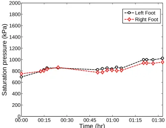
export forces. Saturation pressure (described above) is closely related to the calibration factor.

Therefore, if some sensors damage during walking, the saturation pressure will change and so

320 

this was tracked throughout the trials. Figure 11 shows a sample of saturation pressure record

321 

for one test subject for the pacing frequency of 2.4 Hz. It can be seen that sensor degradation

322 

is small because the saturation pressures over a period of about 1.5 hours remain reasonably

323 

consistent.

324 

00:000 00:15 00:30 00:45 01:00 01:15 01:30

200 400 600 800 1000 1200 1400 1600 1800 2000

Time (hr)

Sat

u

rat

ion pres

s

u

re (k

Pa)

Left Foot Right Foot

325 

Figure 11 Saturation pressure vs. time (hour) for one test subject and pacing frequency of 2.4 Hz.

326 

327 

4. Data Analysis

328 

4.1 Dynamic load factors

329 

Walking forces are commonly described using a Fourier series [24]:

330 

 





0

DLF cos 2

r

p k p k

k

G t W











331 

where Wp = mpg; mp is the pedestrian mass; g is the acceleration due to gravity; fp is the pacing

332 

frequency; and DLFk is the dynamic load factor for the kth harmonic. The phase angle of the

333 

kth harmonic is denoted by φk , and r represents total number of harmonics considered. In this

representation, the harmonic k = 0 corresponds to the static pedestrian weight, and so φ0 = 0 to

335 

give DLF0 = 1. To calculate the DLFs from the GRF measurements, the start and end of the

336 

recorded walking force signals are trimmed such that a signal consists of some even number of

337 

full steps achieved. Then, the DC component is subtracted from the signal and then the signal

338 

is windowed using a Hann window to suppress leakage. The signal is zero-padded afterwards

339 

and transformed into the frequency domain using the Fast Fourier Transform (FFT). The signal

340 

amplitude in the frequency domain is corrected for the side-lobe loss due to using Hann window

341 

[43]. Figure 12 shows all steps to determine dynamic load factor for the exemplary test subject,

342 

highlighting the first four DLFs. Consistent with the literature, the pedestrian force is not

343 

perfectly periodic; in fact, it is a narrow band signal with some of its energy spread to adjacent

344 

frequencies [44], [45]. Phase angles are also found to be more or less uniformly distributed

345 

from 0 to π radians.

346 

2 4 6 8 10 0

1 2

t (s)

G BS

/w

p

(a) _{Original signal}

Trimmed signal

2 4 6 8 10

-0.5 0 0.5

G BS

/w

p

-1

t (s) (b)

0 1 2 3 4

0 0.2 0.4

f/f p

M

agn

it

u

d

e

of

FFT

(c)

Force magnitude Dynamic load factors

348 

Figure 12 Determination of walking DLFs: (a) Tekcsan original and trimmed force signal (b) windowed

349 

trimmed signal (b) Fast Fourier Transform of the trimmed signal with frequency resolution, 0.01 Hz (the

350 

variability in FFT might not be representative of normal walking due to setting the pacing frequency with the

351 

metronome, and some of the energy spread to adjacent frequencies is due to leakage from the use of the Hann

352 

window).

353 

354 

For each trial and surface (rigid and bridge surface), first two DLFs of pedestrian force are

355 

calculated. Then, the mean DLF is taken across the five trials for each test subject for a specific

356 

pacing frequency. Figure 13 illustrates the mean first and second DLF for different frequency

357 

ratios and mass ratios (the grey regions show Kerr’s DLFs [46]). As seen in Figure 13a, for the

358 

resonance case,  = 1, the difference between the mean first DLF of the rigid and bridge

359 

surfaces is significant. As the mass ratio increases, this difference tends to increase. However,

360 

the difference is not monotonically increasing. From Figure 13b, it is clear that, for resonances

361 

by both first and second harmonic,  = 1 and  = 0.5, there is a substantial difference between

second mean DLFs of rigid and bridge surface. Furthermore, the DLFs on the bridge surface

363 

are smaller than those on the rigid surface for  = 1. When becomes far from 1 (i.e.  = 0.87,

364 

0.5), the difference in first DLFs gets smaller, and it seems that the vibrating bridge does not

365 

have a significant effect on the mean DLFs. The second DLFs of the bridge surface are smaller

366 

than those of the rigid surface for both resonance and second harmonic excitation,  = 1 and

367 

= 0.5. Considering then the postulated S2HI effect, the bridge surface DLFs can be expressed

368 

as:

369 

S2HI

DLF



DLF



DLF

370 

which

DLF

DLF

371 

surfaces, respectively;



DLF

372 

caused by the vibration. It should be mentioned that as the test subject gets heavier, this effect

373 

typically becomes more pronounced.

374 

375 

The drop in DLF1 on the lively surface was also found in [47], [23] in which it was explained

376 

as being a consequence of a vibration-induced ‘self-excited force’. This concept suggests that

377 

there are two components combine to give the GRF on the bridge surface,

G

378 

force,

G

G

379 

of what amount of HSI is to be characterized as “self-excited”.

0.3 0.35 0.4 0.45 0.5 0.55 0.6 0.65 0.7 0

0.2 0.4 0.6

DL

F 1



m (%)

(a)

0.3 0.35 0.4 0.45 0.5 0.55 0.6 0.65 0.7

0 0.05 0.1



m (%)

DL

F 2

(b)

BS- = 0.50 RS- = 0.50 BS- = 0.87 RS- = 0.87 BS- = 1.00 RS- = 1.00

381 

Figure 13 Mean dynamic load factor of (a) first harmonic (b) second harmonic versus mass ratio for different

382 

frequency ratios, showing Kerr’s [46] DLF regions (greyed) (RS and BS stand for rigid surface and bridge

383 

surface respectively).

384 

385 

4.2 Simulated and measured vibration response

386 

The analytical model used to simulate vibration response is shown in Figure 14. The pedestrian

387 

is modelled as a force moving at constant velocity and the bridge is modelled as a

simply-388 

supported beam in modal space considering only the first mode of the vibration. The measured

389 

force, G(t), moving at the actual average velocity as recorded in each trial is used in simulations.

390 

As previously mentioned, the bridge frequency and damping are amplitude-dependent, and this

391 

is considered in the numerical model.

392 

394 

Figure 14 Analytical modelling of human-bridge system.

395 

396 

The equation of motion in modal space is [24]:

397 

 

 

 

   

b b b

b

x G t

q t q t q t x vt

M



   

  

&& & (3)

398 

where q, q&, and q&& are the modal displacement, velocity, and acceleration for the first mode of

399 

the bridge;





400 

of the first mode; they are updated for each amplitude of vibration [48];

M



 

401 

modal mass and mode shape; G t

 

402 

surface (

G

G

403 

pedestrian location at time t, while v is the average velocity of the traverse. The modal vibration

404 

response of the bridge is obtained using Newmark- integration. Finally, vibration response of

405 

the bridge in physical coordinates at any location is given by:

406 

     

u x t&& 



407 

where the mode shape can be approximated by a half-sine function [49]:

408 

 

L





  (5)

409 

where L is the bridge length. Figure 15a shows the measured vibration response and simulated

410 

RS, and BS responses at the bridge mid-span for the exemplary test subject. The measured

accelerations are seen to be smaller than that simulated by the numerical model, even when

412 

using the measured induced force to the bridge surface. The difference between the peak

413 

amplitudes of measured and both forms of simulated vibrations for the exemplary test subject

414 

are shown in Figure 15b. The differences between the RS and BS responses as well as between

415 

the measured and BS responses become more and more obvious as the response amplitude

416 

increases. However, these differences have sporadic increasing and decreasing trends. Further,

417 

in this example, the difference is far more significant between measured and BS responses,

418 

than between RS and BS responses.

419 

0 2 4 6 8 10 12

-4 -2 0 2 4

t (s)

a M

(m

/s

2 )

(a)

Measured response Simulated BS response Simulated RS response

0 0.5 1 1.5 2

0 0.2 0.4 0.6 0.8 1

Measured a

peak (m/s 2

)



a p

eak

(m

/s

2 )

(b)

Between measured and BS responses Between RS and BS responses

420 

Figure 15 (a) Measured response (from the experiment), simulated BS, and RS responses (from the numerical

421 

model) (b) differences beetwen peak amplitudes of the responses of (a) – see Figure 2 for meaning.

422 

423 

The maximum of each acceleration time history, amax, is used as a response metric. Maximum

acceleration over a few cycles of vibration, and so response ratios are unaffected by the measure

426 

used. The results are given in Tables 3 (RS responses) and 4 (BS responses), and shown in

427 

Figure 16. The variability of results is low with coefficient of variation up to 0.29 and central

428 

tendencies are therefore meaningful to describe the results.

429 

430 

Table 3. Maximum acceleration response (amax, m/s2) of the numerical model using the measured rigid surface

431 

GRFs.

432 

Test Subject

Mass Ratio, m (%)

Frequency Ratio, 

Trial No.

Mean 1 2 3 4 5

1 0.33

0.50 0.10 0.24 0.18 0.16 0.18 0.17

0.87 0.17 0.19 0.24 0.15 0.19 0.19 1.00 1.13 1.34 1.29 1.53 1.45 1.35

2 0.40

0.50 0.14 0.13 0.16 0.16 0.11 0.14 0.87 0.17 0.18 0.21 0.15 0.15 0.17 1.00 1.38 1.31 1.49 1.52 1.52 1.44

3 0.50

0.50 0.14 0.14 0.14 0.16 0.15 0.15 0.87 0.34 0.23 0.31 0.33 0.23 0.29 1.00 2.06 2.02 1.97 1.79 1.68 1.90

4 0.60

0.50 0.27 0.29 0.25 0.22 0.26 0.26 0.87 0.33 0.31 0.29 0.31 0.32 0.31 1.00 2.98 2.28 3.11 2.95 2.96 2.86

5 0.70

0.50 0.63 0.56 0.65 0.53 0.42 0.56 0.87 0.36 0.38 0.42 0.34 0.42 0.38 1.00 2.19 3.36 1.62 3.48 2.91 2.71

433 

Table 4. Maximum acceleration response (amax, m/s2) of the numerical model using the measured bridge surface

434 

GRFs.

435 

Test Subject

Mass Ratio, m (%)

Frequency Ratio, 

Trial No.

Mean 1 2 3 4 5

1 0.33

0.50 0.22 0.23 0.12 0.24 0.21 0.20

0.87 0.17 0.25 0.22 0.19 0.18 0.20

1.00 1.31 1.42 1.31 1.38 1.34 1.35

2 0.40

0.50 0.09 0.06 0.09 0.07 0.06 0.07

0.87 0.17 0.19 0.16 0.14 0.08 0.15

1.00 1.10 1.53 1.46 1.37 1.27 1.35

0.87 0.37 0.26 0.30 0.26 0.24 0.28

1.00 1.65 1.07 1.76 1.51 1.59 1.52

4 0.60

0.50 0.23 0.20 0.19 0.30 0.27 0.24

0.87 0.27 0.29 0.25 0.22 0.26 0.26

1.00 1.54 1.86 2.42 2.27 2.68 2.15

5 0.70

0.50 0.47 0.49 0.47 0.59 0.65 0.53

0.87 0.29 0.40 0.44 0.32 0.39 0.37

1.00 3.22 3.29 3.62 3.26 3.26 3.33

436 

To perform further analysis and understand the central tendency of the simulated and measured

437 

responses, an average is taken across trials for each test subject with a specific pacing frequency,

438 

and it is shown in the last column of Tables 3 and 4. For  = 1 the RS response is greater than

439 

the BS response for almost all test subjects except for the test subject with mass ratio 0.70%.

440 

The BS response is significantly larger than the measured response for all cases at frequency

441 

ratio of 1. As shown in the experimental-numerical programme (Figure 2), these differences

442 

between RS and BS responses, and between BS and measured responses reflect S2HI and H2SI,

443 

respectively. Hence, excluding S2HI and H2SI overestimates vibration response by up to 32%

444 

and 33%, respectively (see Figure 16c).

445 

446 

The overestimation of vibration response as a result of ignoring both HSI forms may lead to

447 

vibration serviceability assessment failure of a bridge, while it may in truth be serviceable.

448 

Both S2HI and H2SI effects increase as frequency ratio and mass ratio increase (Figure 16c).

449 

For S2HI, it means that its influence on the walking force acting on the bridge surface increases,

450 

both as the vibration amplitude tends to increase and as the test subject gets heavier. For H2SI,

451 

the effects of the test subjects’ mass and pacing frequency support the hypothesis that the

452 

human body can act as a dynamic absorber. When the pacing frequency of the test subject

453 

(absorber frequency) is close to the bridge frequency, the energy dissipated by the pedestrian

increases. Also, as the test subject (absorber) gets heavier, it seems that more energy is damped

455 

out of the bridge. 

456 

457 

0.35 0.4 0.45 0.5 0.55 0.6 0.65 0.7

0 0.5 1

 m (%)

a max

(m

/s

2 )

(a)

Mean measured response Mean RS response Mean BS response

0.35 0.4 0.45 0.5 0.55 0.6 0.65 0.7

0 0.5 1

a max

(m

/s

2 )

 m (%)

(b)

0.35 0.4 0.45 0.5 0.55 0.6 0.65 0.7

0 2 4

a max

(m

/s

2 )

 m (%)

(c)

458 

Figure 16 Mean maximum acceleration for frequency ratio of: (a) 0.50 (b) 0.87 (c) 1. See Figure 2 to understand

459 

why the blue (BS) to black (measured) lines reflects the effect of H2SI and red (RS) to blue, that of S2HI.

460 

461 

5. Statistical Tests

462 

In section 4.2, it was shown that the differences between mean responses are large at resonance.

463 

These differences are an indication of HSI as per Figure 2. However, two important caveats

464 

must be considered regarding the results. First, a small number of five trials for each test subject

465 

and pacing frequency was used to calculate the mean maximum acceleration response for the

466 

simulated RS and BS vibration response and measured vibration response. The question then

467 

mean vibration responses. In other words, are the differences in means by chance or

469 

representative of the population of responses as a whole? To answer this, parametric statistical

470 

hypothesis testing is used. Second, careful consideration must be given to measurement

471 

inaccuracies input to the numerical model which consequently influence the simulated

472 

vibration responses. To quantify this, the input parameters are described in terms of probability

473 

density functions (PDFs) and Monte Carlo simulations of output responses conducted. This

474 

allows a broader understanding of the differences between the results, and hence the

475 

quantitative influence of HSI in a probabilistic sense.

476 

477 

5.1 Parametric test (hypothesis test)

478 

A parametric test makes assumptions about the underlying distribution of the population from

479 

which the sample is being drawn. The population distribution of responses is assumed to be

480 

normal, which can be reasonably justified through the central limit theorem [50]. According to

481 

the experimental-numerical programme (Figure 2), the null, H0, and alternative hypotheses, H1,

482 

for each HSI form are given as:

483 

1) S2HI:

484 

0

1

: 0

: 0

RS BS RS BS

H R R

H R R

  

 _{ }

 (6)

485 

2) H2SI:

486 

0

1

: 0

: 0

BS M BS M

H R R

H R R

  



 

 (7)

487 

where

R

R

R

488 

measured cases respectively for a large population of trials. If null hypothesis, H0, is correct it

489 

means that HSI is not significant, and that the difference in the means of two small samples are

by chance; otherwise, the alternative hypothesis, H1, is more likely and HSI exists in the

491 

population of vibration responses.

492 

493 

When performing the hypothesis test, no HSI (null hypothesis) might be reached or two errors

494 

could be made: incorrectly accepting HSI when it does not exist (error of the first kind) or

495 

rejecting it when it does exist (error of the second kind). It is desirable to minimize the

496 

probabilities of the two types of error. However, these errors cannot be controlled. Therefore,

497 

a level of significance, , is assigned to the probability of incorrectly accepting HSI when it

498 

does not exist and then the error due to rejecting HSI when it does exist is minimized. The

499 

standard way to remove the arbitrary choice of  is to report the p-value of the test, defined as

500 

the smallest level of significance leading to accepting the alternative hypothesis (i.e. that HSI

501 

exists). The p-value gives an idea of how strongly the data contradicts the hypothesis that there

502 

is no HSI of any form. A small p-value shows that the mean response metrics are highly likely

503 

to be different, and hence HSI exists.

504 

505 

To test the difference between the two samples for each form of HSI (see Figure 2 and

506 

equations (6) and (7)), the two-sided independent sample Student’s t-test is used, with equal

507 

variances assumed for both populations. Table 5 summarizes the hypothesis test results for

508 

both HSI forms for each pacing frequency, as assessed using the maximum acceleration

509 

response metric (Tables 1, 3, and 4). It is clear that HSI only has significance for the β = 1 case

510 

(for which p-values are small) while for the other frequency ratios, HSI mostly does not have

511 

a statistically significant effect on the result. Considering then just the resonant case, for both

512 

HSI forms, it can be seen that higher mass ratios mostly gives smaller p-values. This means

513 

that the effect of HSI effect increases with mass ratio (as may be expected). However, typically

514 

p-values resulting from H2SI, especially for heavy test subjects, are smaller than those of S2HI,

indicating that the effect of HSI on the dynamic properties of the system is more pronounced

516 

than the effect of the structure on the pedestrian walking force. There are some unexpected

517 

cases though for the mass ratios of 0.40% and 0.50%. Nevertheless, overall for the resonant

518 

case ( = 1), the results give strong support to the existence of H2SI, and somewhat weaker

519 

support to S2HI and show that the mass ratio is an important factor.

520 

521 

Table 5. p-values for the two postulated forms of HSI from the t-test for the maximum acceleration metric.

522 

Test

Subject μm (%)

 = 0.5  = 0.87  = 1

S2HI H2SI S2HI H2SI S2HI H2SI

1 0.33 0.33 0.40 0.52 0.35 0.96 0.29

2 0.40 0.41 0.54 0.30 0.10 0.29 0.67

3 0.50 0.75 0.19 0.95 0.25 0.02 0.17

4 0.60 0.43 0.24 0.72 0.92 0.05 0.02

5 0.70 _{0.67 1.00 0.63 0.97 0.13 0.00}

523 

5.2 Non-parametric test (Monte Carlo Simulation)

524 

Non-parametric testing is used to determine the effects of measurement and model errors on

525 

the numerical model vibration response, and hence the conclusions drawn from these results.

526 

Such errors could affect the HSI quantification, since the postulated HSI forms are defined in

527 

terms of differences between simulated and measured responses. Figure 17 illustrates a

528 

schematic view of potential errors in the experimental-numerical programme (also refer to

529 

Figure 2). It includes the real bridge, numerical model inputs and outputs, as well as errors.

530 

The first type of error is measurement error.

G

531 

inputted into the real bridge. RM is the measured response of the bridge with possible error, a,

532 

for one walking trial. This error is assumed negligible as the accelerometers used to measure

533 

the bridge response (Honeywell QA750) are of very high quality, with very low noise floor

534 

and output frequency response down to DC. The final measurement error is due to the GRF

measurement system, TekScan, denoted G, which influences the measured pedestrian forces,

536 

GBS and GRS.

537 

538 

539 

Figure 17 Schematic view of errors for: (a) real bridge (b) numerical model.

540 

541 

The second type of error is the error of the numerical model, NM, which reflects the ability of

542 

the (simple) model to replicate reality. This error emanates from many possible sources which

543 

do occur but are not adequately captured in the model, such as the actual damping, frequency,

544 

mass, frictions/nonlinearities, nonlinear material behaviour, etc. In particular, the effects of the

545 

bridge damping and frequency are significant at resonance: small changes in these strongly

546 

affect the vibration response and so these are considered in detail. Each considered model

547 

parameter error is defined as:

548 

 

X

   (8)

549 

where XBM is the benchmark value for the parameter, X. For the bridge damping and frequency,

550 

the free vibration results at the end of each trial were taken as the benchmark values, which is

reasonable since any a is extremely small as noted above. Thus, the errors are estimated for

552 

the bridge damping and frequency using equation (8). Kernel density estimation is then used

553 

to estimate the PDF of the errors for each variable [51]. Figure 18 shows the PDFs of the errors

554 

for bridge frequency and damping.

555 

556 

Figure 18 Probability density of bridge: (a) frequency (b) damping.

557 

558 

For the GRFs, the results of the force plate are treated as the benchmark or ‘true’ values. The

559 

Tekscan system generally gives different force estimate. To model the true force from the

560 

Tekscan measurements, the Tekscan error is analysed statistically. Since the sample rate is the

561 

same for both the force plate and Tekscan, time is indicated by the index, i. Index j is used to

562 

-0.050 0 0.05

10 20 30 40 50

P

robabi

lit

y

densi

ty

 (

b )

(b)

-0.020 -0.01 0 0.01 0.02

100 200 300 400 500

(a)

P

ro

b

a

b

ility

d

e

n

s

ity

 (f

denote a specific trial of which there are N. The Tekscan measurement relative error for trial j

563 

at time i is:

564 

FP TS ij ij

ij TS

ij

G G

G

   (9)

565 

Figure 19a shows the histogram of ij for all trials, and Figure 19b illustrates the probability

566 

density of the relative errors using Kernel density estimation [51]. As a conservative estimation

567 

of the Tekscan error, this probability density function is used to generate relative random errors,

568 

i



569 





FP TS

i i i

G  



570 

Finally, randomly generated representative force plate footsteps are combined to create a

571 

continuous force plate GRF.

572 

573 

Using this procedure for input force, and PDFs (Figure 18) for bridge frequency, and damping,

574 

104 _{Monte Carlo simulations (MCSs) are performed to determine the variability of results due}

575 

to these possible errors. It is emphasized that the PDFs used are nonparametric (i.e. directly

576 

those of Figures 18 and 19b), and so no additional error is introduced by assuming a parametric

577 

PDF form (e.g. normal, lognormal).

-0.10 -0.05 0 0.05 0.1 0.15 0.2 0.25 0.3 0.35 10

20 30 40 50 60 70

 (G)

Fr

e

q

ue

nc

y

o

f oc

c

u

rr

en

c

e

(a)

-0.20 -0.1 0 0.1 0.2 0.3 0.4 0.5 0.5

1 1.5 2 2.5 3 3.5 4

P

robabi

lit

y d

ensi

ty

 (G) (b)

579 

Figure 19. Tekscan measurement relative error: (a) histogram (b) probability density.

580 

581 

By way of example, Figure 20 shows the resulting histograms for possible RS and BS responses

582 

considering the model errors, along with the actual corresponding measured response for the

583 

exemplary test subject. The figure suggests that the RS and BS response distributions are

584 

strongly biased with respect to the measurement. This is due to the very wide error distribution

585 

taken for the Tekscan error; unfortunately no better error model is available. Nevertheless, in

586 

a relative sense, there is a difference between the distributions for RS and BS forces. According

587 

to the experimental-numerical framework of Figure 2, this then, is the influence of HSI.

Further, the distance between the mean and measurement reflects to some extent the error of

589 

the state-of-the-art practice (Figure 2).

590 

591 

592 

Figure 20 Histograms for RS and BS responses from MCS which considers possible measurement errors, and

593 

the corresponding measured vibration response.

594 

595 

To quantify the HSI effect, the relative difference between the vibration responses is defined

596 

based again on Figure 2. Thus, for S2HI we have:

597 

S2HI RS BS

M R



 R R (11)

598 

and for H2SI:

599 

H2SI BS M

M R R



 R (12)

600 

in which

R

R

601 

surfaces, respectively obtained from MCS. Then, PDFs are constructed for each trial

602 

individually, as well as for the group of 5 trials as a whole (merged trials). Figure 21 shows the

603 

PDFs for the exemplary test subject for each individual trial and the merged trials. It is clear

604 

1.5 2 2.5 3 3.5 4 4.5

0 100 200 300 400 500 600

R (m/s2)

N

u

m

ber

of

M

C

S

RS response BS response

that most of the randomly realized -values for both HSI forms are non-zero and positive,

605 

indicating the relative influence of HSI. The grey filled areas represent the probability of HSI

606 

non-existence or negative effect (negative side of the probability curves). In this example, this

607 

probability is 20% and 5% for S2HI and H2SI respectively, again reflecting that both are likely

608 

to exist and that H2SI is by far the stronger effect.

609 

610 

Figure 21 Probability density for the exemplary test subject at resonance for (a) S2HI (b) H2SI.

611 

612 

613 

The effects of both HSI forms on vibration response can be given as:

614 

615 

1 RS M

R

R 

  (13)

where,

617 

HSI S2HI H2SI

  

618 

The vibration response based on RS measurements is reduced by a factor to reach the measured

619 

vibration response. The most likely values of





620 

the PDFs similar to Figure 21. These values are 0.21 and 0.27 for the exemplary test subject

621 

(Figure 21) giving a combined factor of 0.67 (as just one example). That is, the measured

622 

response is 67% of that estimated using rigid surface GRFs and a moving force numerical

623 

model (even allowing for amplitude-dependent damping). Table 6 shows these results for each

624 

test subject for the case at resonance only, since this is when HSI has most effect. The results

625 

show that HSI has a significant effect, and it increases with mass ratio. With further

626 

experiments, results of this nature could be used to provide more accurate vibration

627 

serviceability models that account for HSI.

628 

629 

Table 6. Relative and combined influence of HSI types (refer to equations (13) and (14)).

630 

Test Subject μμμm (%) S2HI H2SI HSI RM/RRS

1 0.33 0.03 0.02 0.05 0.95

2 0.40 0.03 0.04 0.07 0.93

3 0.50 0.12 0.17 0.29 0.77

4 0.60 0.21 0.27 0.48 0.67

5 0.70 0.10 0.28 0.38 0.72

631 

6. Conclusions

632 

In this paper, the human-structure interaction phenomenon was quantified using a novel

633 

experimental-numerical approach. The imparted footfall force to both rigid and bridge surface

634 

was measured along with the resulting bridge response. The moving force model was adopted

635 

to simulate vibration as a commonly-used model in design codes which ignores

human-636 

structure interaction. The difference between simulated and measured responses as well as the

difference between dynamic load factors of the forces on the rigid and bridge surface were used

638 

as criteria to evaluate HSI existence.

639 

640 

It was found that human-structure dynamic interaction is associated both with the forces that

641 

excite the structure (S2HI) and with the corresponding influence of humans on the dynamic

642 

properties of the structure they occupy (H2SI). H2SI is found to be a far stronger influence than

643 

S2HI for the bridge studied. The intensity of both S2HI and H2SI is found to increase as the

644 

mass ratio between the human and structure increases. At resonance, where vibration amplitude

645 

reaches its peak, the HSI effects are the most pronounced. The results of parametric statistical

646 

hypothesis testing show that HSI is of statistical significance, and H2SI is very likely in

647 

particular. Furthermore, non-parametric testing was done to see the effects of numerical model

648 

and measurement errors on HSI existence. It shows that HSI remains of statistical significance

649 

even accounting for numerical model and measurement errors. Similar to the parametric test,

650 

it is found that H2SI is more statistically significant than S2HI. This approach enabled a

651 

probabilistic quantification of both HSI effects, as well as their combined effect. Such an

652 

approach could prove useful in adapting the moving force model to give results that compare

653 

better to measurements.

654 

655 

The Warwick Bridge has a low pedestrian-to-bridge mass ratio, up to 0.7% in this study. For

656 

bridges with higher mass ratios, the intensity of H2SI might be even more significant and

657 

pedestrian effects on dynamic properties of the system could be even more pronounced than

658 

bridge vibration effects on pedestrian walking force.

659 

660 

This study is a beneficial step forward towards quantifying HSI. It introduces a novel

661 

framework which is a combination of an experimental and numerical approach to investigate