Original citation:
Petrella, Ivan, Rossin, R. and Santoro, Emiliano. (2017) Monetary policy with sectoral trade-offs. The Scandinavian Journal of Economics.
Permanent WRAP URL:
http://wrap.warwick.ac.uk/86227
Copyright and reuse:
The Warwick Research Archive Portal (WRAP) makes this work by researchers of the University of Warwick available open access under the following conditions. Copyright © and all moral rights to the version of the paper presented here belong to the individual author(s) and/or other copyright owners. To the extent reasonable and practicable the material made available in WRAP has been checked for eligibility before being made available.
Copies of full items can be used for personal research or study, educational, or not-for profit purposes without prior permission or charge. Provided that the authors, title and full bibliographic details are credited, a hyperlink and/or URL is given for the original metadata page and the content is not changed in any way.
Publisher’s statement:
"This is the peer reviewed version of the following Petrella, Ivan, Rossin, R. and Santoro, Emiliano. (2017) Monetary policy with sectoral trade-offs. The Scandinavian Journal of Economics. which has been published in final form at http://doi.org/10.1111/sjoe.12266. This article may be used for non-commercial purposes in accordance with Wiley Terms and Conditions for Self-Archiving."
A note on versions:
The version presented here may differ from the published version or, version of record, if you wish to cite this item you are advised to consult the publisher’s version. Please see the ‘permanent WRAP URL’ above for details on accessing the published version and note that access may require a subscription.
Monetary Policy with Sectoral Trade-o¤s
IVAN PETRELLA RAFFAELE ROSSIy EMILIANO SANTOROz
December 5, 2016
Abstract
We formulate a two-sector New Keynesian economy that features sectoral heterogeneity along three main dimensions: price stickiness, consumption goods durability, and the inter-sectoral trade of input materials. The combination of these factors deeply a¤ects inter-sectoral and intra-sectoral stabilization. In this context, we examine the welfare properties of simple rules that adjust the policy rate in response to the output gap and alternative measures of …nal goods price in‡ation. Aggregating durable and non-durable goods prices depending on the relative frequency of sectoral price-setting may induce a severe bias. Due to factor demand linkages, the cost of production in one sector is in‡uenced by price-setting in the other sector of the economy. As a result, measures of aggregate in‡ation that weigh sectoral price dynamics based on the relative degree of price rigidity do not allow the central bank to keep track of the e¤ective speeds of sectoral price adjustment.
JEL classi…cation: E23, E32, E52
Keywords: Durable Goods, Input-Output Interactions, Monetary Policy, Interest Rate Rules
Warwick Business School and CEPR. Address: Warwick Business School, The University of Warwick, Coventry, CV4 7AL, UK.E-mail: [email protected].
yDepartment of Economics, University of Manchester. Address: Manchester M13 9PL, UK. E-mail: [email protected].
1
Introduction
Along with major di¤erences in the time span over which they yield consumer utility, durable and
non-durable consumption goods are characterized by deep peculiarities in their production and
price-setting. Such structural traits are paramount to the monetary transmission mechanism (Barskyet al.,
2007) and need to be accounted for when designing realistic multi-sector economies.1 From a normative
viewpoint, the literature available to date has extensively reported that sectoral heterogeneity presents
the central bank with a nontrivial trade-o¤. With a single instrument, the policy maker cannot
replicate the frictionless equilibrium allocation in each sector of the economy. This principle applies
whenever sectoral discrepancies concern at least one of the following characteristics: price rigidity
(Aoki, 2001), durability of di¤erent consumption goods (Erceg and Levin, 2006), inter-sectoral trade
of input materials (Huang and Liu, 2005; Petrella and Santoro, 2011).2 All these factors are widely
recognized to be major determinants of the relative price of goods produced by di¤erent sectors, which
in turn exerts a strong in‡uence on aggregate in‡ation (Reis and Watson, 2010). Therefore, drawing
predictions based on single-sector models fails to re‡ect the underlying sources of aggregate in‡ation
dynamics.3 The present study addresses these issues from a normative perspective, integrating the
main sources of sectoral heterogeneity into a two-sector New Keynesian economy.
In the economy under examination the monetary authority cannot attain the Pareto optimal
allocation consistent with the full stabilization of sectoral productions and in‡ation rates, even when
distortions in the labor market (i.e., imperfect labor mobility) and the goods market (i.e., monopolistic
competition) are removed. Thus, we turn our attention to policy strategies capable of attaining
second best outcomes. To this end, we derive an appropriate welfare metric through a quadratic
approximation of households’utility and assume that the central bank pursues its policy under timeless
perspective commitment (Woodford, 1999, 2003). In doing so, the policy maker needs to account for
some distinctive features that a¤ect both inter-sectoral and intra-sectoral stabilization. As for the …rst
aspect, Erceg and Levin (2006) showed that durables are much more interest rate-sensitive than
non-durables, even though they feature a relatively lower expenditure share of households’consumption.4
This property exacerbates the trade-o¤ entailed in stabilizing real activity in the two sectors, as
1Bouakez et al. (2014, 2009) have shown that heterogeneity in price rigidity is a crucial factor to understand why
sectoral in‡ation rates do not feature analogous responses to monetary policy shocks, while the degree of durability has important implications for explaining sectoral output responses.
2Though other forms of sectoral heterogeneity could be envisaged, we focus on the most pervasive ones that have
been explored by the literature available to date.
3Petrella and Santoro (2012) report substantial heterogeneity in sectoral in‡ation dynamics, with variations in the
income share of input materials traded among sectors representing a key driver.
4The pronounced magnitude of durables’ response depends on two inherent features of this type of good: …rst, the
compared with models featuring two non-durable goods. In the present work we show that factor
demand linkages also play a major role in shaping the behavior of the relative price. In fact, the
cross-industry ‡ow of input materials is responsible for magnifying negative sectoral co-movement in
the face of monetary policy innovations. As for intra-sectoral stabilization, it is important to recall
that intermediate goods reduce the slope of the sectoral production schedules, as compared with
models that neglect the presence of input materials (Petrella et al., 2014). This property limits the
pass-through from the sectoral marginal costs to the respective rates of in‡ation. As a result, the
central bank may attach greater importance to limiting ‡uctuations in the sectoral production gaps,
as compared with models that disregard the role of input materials.
We assess the capability of simple interest-rate feedback rules to mimic the optimal policy
bench-mark. One obvious advantage of these policy functions is to abstract from the stringent informational
requirements of the rule under timeless perspective. Moreover, while the model-consistent welfare
criterion involves sector-speci…c variables, we assume that the policy rate is adjusted in response to
broad measures of real activity and prices. A major problem we are confronted with when designing
optimal interest rate rules for multi-sector economies is to …nd the most appropriate in‡ation rate
to target (see, e.g., Huang and Liu, 2005). To this end, the model lends itself to account for three
options: (i) aggregate in‡ation, according to which the sectoral in‡ation rates are aggregated
depend-ing on the relative size of each sector; (ii) sticky-price in‡ation, which weighs sectoral price dynamics
depending on both the relative size and the relative degree of rigidity in price-setting of each sector;
(iii) a measure of aggregate in‡ation that removes ‡uctuations in the price of oil from changes in
the general price level. It is important to stress that sticky-price in‡ation is typically believed to
be the most appropriate variable to monitor relative price changes in multi-sector environments that
feature heterogeneous speeds of sectoral price adjustment (Woodford, 2003, pp. 435-443). Also policy
makers display increasing interest in this type of measures. For instance, the Atlanta FED regularly
publishes its Sticky Price Index, which sorts the components of the consumer price index (CPI) into
either ‡exible or sticky (slow to change) categories, based on the frequency of their price adjustment.
Also Eusepi, Hobijn, and Tambalotti (2011) have recently constructed a cost-of-nominal-distortions
index (CONDI), whose weights depend on sectoral price stickiness.
The analysis of the interest-rate feedback rules delivers one key …nding: targeting sticky-price
in‡ation produces a higher loss of social welfare, as compared with reacting to aggregate in‡ation
or to a measure of price changes that excludes oil price dynamics. This result crucially rests on the
presence of inter-sectoral production linkages and the cross-industry externalities they generate in
inherit considerable extrinsic persistence through the in‡uence of non-durable goods prices on their
marginal cost of production. For the same reason, price stickiness in the non-durable goods sector is
partly attenuated through the inter-sectoral input-output channel. As a result, aggregating durable
and non-durable in‡ation depending on the relative frequency of sectoral price-setting may induce a
severe bias, as the central bank does not properly keep track of the e¤ective speeds of sectoral price
adjustment. A similar issue emerges when taking the perspective of a delegated central banker that
balances the stabilization of the output gap with that of an aggregate measure of price changes. In
this case, weighing sectoral in‡ations based on their relative degree of price rigidity does not allow
the central banker to take into account the intra-sectoral stabilization trade-o¤ in the durable goods
sector. In fact, while the dual mandate implicitly attributes a sizeable weight to stabilizing the gross
production of durables, their in‡ation rate is virtually neglected by measures of sticky-price in‡ation,
despite their marginal cost depends on the cost borne to buy input materials from the non-durable
goods sector.
The remainder of the paper is laid out as follows: Section 2 introduces the theoretical setting;
Section 3 reports the calibration of the model economy; Section 4 discusses the implementation of the
optimal monetary policy; Section 5 examines the stabilization properties of alternative regimes for
monetary policy-making. Section 6 concludes.
2
The Model
We develop a New Keynesian DSGE model with two sectors that produce durable and non-durable
goods, respectively. The model economy is populated by a large number of in…nitely-lived households.
Each of them is endowed with one unit of time and derives utility from consuming of durable goods,
non-durable goods and leisure.
The production technology of both sectors employs labor, input materials and oil. The two
sectors are connected through factor demand linkages.5 In this respect, the inter-sectoral ‡ows of
intermediate goods are determined by the input-output matrix of the economy, which is based on the
implicit assumption that – once goods enter the production process – they only last a single period,
vanishing within the assembled good. Despite appearing somewhat counterintuitive, this principle also
applies to durables being used as input materials.6 One example should help us clarifying this point.
According to the Standard Industry Classi…cation adopted by the Bureau of Economic Analysis,
5Throughout the paper we will refer to ‘factor demand linkages’as indicating cross-industry ‡ows of input materials.
Should a speci…c feature of the model economy be essentially determined by the use of intermediate goods in the production process (i.e., inter-sectoral relationships are not essential), we will explicitly refer to ‘input materials’.
6
group 322 identi…es the establishments that are primarily engaged in manufacturing glass containers
for commercial packing and bottling. These are key primary inputs for the food and beverage sector
(group 20), which produces non-durable goods. Another typical example is group 3411 in the durable
goods sector, which includes the producers of metal cans. These are among the main suppliers of
…rms included in group 203 (i.e., canned foods), whose …nal product is regarded as a non-durable
good.
Inter-sectoral production linkages do not only represent a salient feature of multi-sector economies,
one that has a crucial role for understanding the transmission of shocks to the economy (Holly and
Petrella, 2012). In fact, they should also be seen as essential building blocks of business cycle models
that aim at generating realistic degrees of sectoral output volatility and co-movement.7 In connection
with the speci…c context we examine, it is well known that sticky-price models incorporating sectoral
heterogeneity in price stickiness –usually in the form of sticky non-durable goods prices and ‡exible
prices of durables – cannot generate positive sectoral co-movement in the face of monetary policy
innovations (Barskyet al., 2007). Inter-sectoral production linkages have been successfully introduced
as a remedy to this lack of co-movement (Bouakez et al., 2011; Sudo, 2012; Di Pace, 2011).
2.1 Consumers
Households derive their income from supplying labor to the production sectors, investing in bonds,
and from the stream of pro…ts generated in the production sectors. Their consumption preferences
are de…ned overHt–a composite of non-durable goods (Ctn) and an ‘e¤ective’stock of durable goods
(Dt) –as well as labor,Lt. They maximize the expected present discounted value of their utility:
E0
1
X
t=0
tU(H
t; Lt); (1)
whereHt= (Ctn) nDtd, n and d denote the expenditure shares on non-durable and durable goods
(so that n+ d = 1) and is the discount factor. We assume that the representative household’s
period utility function takes the form:
U(Ht; Lt) =
Ht1
1 %
L1+t v
1 +v; % >0 (2)
7Horvath (1998, 2000) and Carvalho (2009) show that cross-industry ‡ows of input materials can reinforce the e¤ect
where is the inverse of the intertemporal elasticity of substitution andvis the inverse of the Frisch
elasticity of labor supply. Durable goods are accumulated according to the following law of motion:
Dt=Ctd+ (1 )Dt 1; (3)
where is the depreciation factor. The e¤ective stock of durables scales the e¤ect of a quadratic cost
of adjustment (see, e.g., Bernanke, 1985):8
Dt=Dt
2
(Dt Dt 1)2
D ; 0; (4)
where Ddenotes the steady state stock of durable consumption goods.
The following sequence of (nominal) budget constraints applies:
X
i=fn;dg
PtiCti+Bt=Rt 1Bt 1+ X
i=fn;dg
WtiLit+ X
i=fn;dg i
t Tt; (5)
where Bt denotes a one-period risk-free nominal bond remunerated at the gross risk-free rate Rt,
Wti denotes the nominal wage rate in sector i = fn; dg and Tt denotes a lump-sum tax paid to
the government. The term nt + dt captures the nominal ‡ow of dividends from both sectors of
production.
We assume that labor can be either supplied to sectornor sectord, according to a CES aggregator:
Lt=
1
(Lnt)1+ + (1 ) 1 Ldt
1+ 1+
; (6)
where denotes the elasticity of substitution in labor supply, and is the steady state ratio of labor
supply in the non-durable goods sector over total labor supply (i.e., =Ln=L). This functional form
conveniently allows us to account for di¤erent degrees of labor mobility between sectors, depending
on .9 To see this we report the equilibrium relationship that governs inter-sectoral mobility. This
8Including an adjustment cost of the stock of durables allows us to obtain results in line with the empirical evidence on
the behavior of durable consumption over the business cycle. King and Thomas (2006) show how the partial adjustment mechanism helps accounting for the aggregate e¤ects of discrete and occasional changes in durables consumption.
9
can be obtained from the …rst order conditions with respect to Lnt and Ldt:10
Wtn Wd t
= 1
1
Lnt Ld t
1
; (7)
For = 0 labor is prevented from moving across sectors. For ! 1workers devote all time to the
sector paying the highest wage. Hence, at the margin, all sectors pay the same hourly wage and perfect
labor mobility is attained. For < 1 hours worked are not perfect substitutes. An interpretation
of this is that workers have a preference for diversity of labor and would prefer working closer to an
equal number of hours in each sector, even in the presence of wage discrepancies.11 This assumption
also re‡ects the common observation that human capital tends to be sector-speci…c in the short run
(see, e.g., Matsuyama, 1992; Wacziarg and Wallack, 2004). In this respect, the CES aggregator in
(6) implies that labor market frictions are neutralized in the steady state, so that the ine¢ ciency
associated with sectoral wage discrepancies is only temporary.
2.2 Producers
The production side of the economy consists of two distinct sectors producing durable (sector d) and
non-durable goods (sectorn). Each sector is composed of a continuum of …rms producing di¤erentiated
products. Let Ytn (Ytd) denote gross output of the non-durable (durable) goods sector:
Yti = "Z 1
0
Yf ti
"it 1
"it df # "it
"it 1
; i=fn; dg (8)
where"itdenotes the time-varying elasticity of substitution between di¤erentiated goods in the
produc-tion composite of sectori=fn; dg. Each production composite is produced in the ‘aggregator’sector
operating under perfect competition. The fth …rm in sectorifaces the following demand schedule:
Yf ti = P
i f t
Pti
! "i t
Yti; i=fn; dg (9)
1 0
The …rst order conditions from consumers’optimization are available in Appendix A.
1 1Horvath (2000) motivates a similar speci…cation based on the desire to capture some degree of sector-speci…city
where Pti is the price of the composite good in the ith sector. From (8) and (9) the relationship
between the …rm-speci…c and the sector-speci…c price is:
Pti = Z 1
0
Pf ti 1 "
i t
df
1 1 "it
; i=fn; dg: (10)
The production technology of a generic …rm f in sector iemploys input materials produced by both
sectors in the economy, labor and oil:12
Yf ti =Zti
2
4 M
ni f t
ni
Mf tdi di
ni
ni
di
di
3 5
M i
Lif t Li Of ti Oi (11)
M i+ Li+ Oi = 1; i=fn; dg
whereZti (i=fn; dg) is a sector-speci…c productivity shock,Lif t denotes the number of hours worked
in the fth …rm of sectori,Mf tji (j=fn; dg) denotes material inputs produced in sectorj and supplied
to …rmf in sectori,Of ti is the amount of oil employed in the production of the same …rmf. Moreover,
ij (i; j=fn; dg) denotes the generic element of the (2 2) input-output matrix and corresponds to
the steady state share of total intermediate goods used in the production of sector j and supplied by
sector i.13
Material inputs are combined according to a CES aggregator:
Mf tji= Z 1
0
Mkf;tji ("
j t 1)="
j t
dk
"jt=("jt 1)
; (12)
where
n
Mkf;tji
o
k2[0;1] is a sequence of intermediate inputs produced in sector j by …rm k, which are 1 2The production technology does not feature physical capital. There are both practical and technical reasons for this
choice. First, capital only accounts for 16% of the total cost of production, followed by labor (34%) and intermediate goods (50%) (source: Dale Jorgenson’s data on input expenditures by US industries). Second, from a normative viewpoint Woodford (2003) and Schmitt-Grohe and Uribe (2007) show that the key policy prescriptions for the New Keynesian framework are not a¤ected by the presence of capital in the production technology. Third, as it will be clear from Section 4, in the present setting we are able to report a compact welfare criterion that allows for a clear understanding of the stabilization trade-o¤s involved by the two-sector economy. By contrast, in the presence of capital accumulation, the welfare loss would not retain the same properties (see Edge, 2003 for the derivation of a utility-based welfare function in a model with endogenous capital accumulation). Fourth, in connection with the speci…c two-sector framework we examine, the transmission channel embodied by sectoral production linkages is not qualitatively a¤ected by the presence of physical capital, as it has been discussed by Sudo (2012). All in all, including capital in the production technology would not alter the key transmission mechanisms of this framework, while rendering the normative analysis more convoluted.
1 3The input-output matrix is normalized, so that the elements of each column sum up to one: P
j=fn;dg jn= 1(and
P
employed in the production process of …rmf in sectori.
Firms in both sectors set prices given the demand functions reported in (9). They are also assumed
to be able to adjust their price with probability 1 i in each period. When they are able to do so,
they set the price that maximizes expected pro…ts:
max
Pi f t
Et 1
X
s=0
( i)s t+s Pf ti +s(1 + i) M Cf ti +s Yf ti+s; i=fn; dg (13)
where t+s is the stochastic discount factor consistent with households’ maximizing behavior, i is
a subsidy to producers in sector i, whileM Cf si denotes the marginal cost of production of …rmf in
sector i. The optimal pricing choice, given the sequence Ptn; Ptd; Ytn; Ytd , reads as:
Pif t= "
i t
"i
t 1 (1 + i)
EtP1s=0( i)s t+sM Cf ti +sYf ti+s
EtP1s=0( i)s t+sYf ti+s
; i=fn; dg: (14)
Note that assuming time-varying elasticities of substitution translates into sectoral cost-push shocks
that allow us to account for sector-speci…c shift parameters in the supply schedules.
In every period each …rm solves a cost minimization problem to meet demand at its stated price.
The …rst order conditions from this problem result in the following relationships:
M Cf ti Yf ti = W
i tLif t
Li
= StO
i f t
Oi
= P
n t Mf tni M i ni
= P
d tMf tdi M i di
; i=fn; dg: (15)
whereSt is the nominal price of imported oil in domestic currency. It is useful to express the sectoral
real marginal cost as a function of the relative price and the real wage prevailing in each sector
i; j =fn; dg,i6=j:
M Cti Pti =
Qit ji M i
RWti Li
Sti Oi M i
M i
Li
Li
Oi
Oi Zti
; (16)
whereSit=St=Pti denotes the price of oil relative to that of goods produced in sectori,RWti=Wti=Pti
is the real wage in sector i and Qi
t denotes the price of sector i relative to that of sector j. Since
Qnt = Qdt 1, in what follows we normalize so as to have a single relative priceQt=Ptn=Ptd. Equation
(16) makes it clear that the relative price exerts a direct e¤ect on the real marginal cost of each sector,
the ith sector the absolute impact ofQtonM Cti=Pti is related to the importance of the other sector as
input supplier, i.e. on the magnitude of the o¤-diagonal elements in the input-output matrix ( ndand
dn). This is a distinctive feature of the framework we deal with, one that has crucial implications
for monetary policy-making. By contrast, in traditional multi-sector models without factor demand
linkages the relative price primarily a¤ects the extent to which consumers substitute durables for
non-durables.
2.3 Market Clearing
The production allocation at the sectoral level is such that
PtiYti =Pti Cti+Mtin+Mtid +StOit; i=fn; dg (17)
Equation (17) implies that sectoral gross production in nominal terms includes the value of
con-sumption and intermediate goods employed in either sector, as well as the value of imported oil.14
Moreover, oil market clearing requires that the sum of oil imported by both sectors equals its supply:
Ont +Otd=Ot;
where Ot is exogenous15 and described by an autoregressive process of order one (see Bodenstein et
al., 2008).
2.4 The Government and the Monetary Authority
The government serves two purposes in the economy. First, it taxes households and provides subsidies
to …rms, so as to eliminate distortions arising from monopolistic competition in the markets for both
classes of consumption goods. This task is pursued via lump-sum taxes that maintain a balanced
…scal budget. Second, the government delegates monetary policy to an independent central bank. In
this respect, we initially assume that the short-term nominal interest rate is used as the instrument
of monetary policy and the policy maker is able to pre-commit to a time-invariant rule. We then
explore the properties of interest rate rules whose reaction coe¢ cients to output and in‡ation are
1 4
Implicitly, part of the domestic production is exported so as to cover the cost of the imported oil (i.e.,PtiEit=StOit, whereEi
t denotes the exports of sectori). This structure is similar to the one envisaged by Blanchard and Galí (2007), though they also allow for a portion of imported oil to be used for consumption purposes.
1 5
computed so as to minimize a quadratic welfare function consistent with consumers’ utility, as well
as the implications of delegating monetary policy to a central banker with di¤erent preferences for
output and in‡ation stabilization, as compared with the general public.
3
Solution and Calibration
To solve the model, we log-linearize behavioral equations and resource constraints around the
non-stochastic steady state and take the percentage deviation from their counterparts under ‡exible prices.
The di¤erence between log-variables under sticky prices and their linearized steady state is denoted by
the symbol "^", while we use " " to denote percent deviations of variables in the e¢ cient equilibrium
(i.e., ‡exible prices and constant elasticities of substitution) from the corresponding steady state value.
Finally, we use "~" to denote the di¤erence between linearized variables under sticky prices and their
counterparts in the e¢ cient equilibrium.16
The model is calibrated at a quarterly frequency. We set = 0:993 and = 2. The inverse of
the Frisch elasticity of labor supply, v, is set to 3, while = 1, so as to account for limited labor
mobility between sectors. As for the parameters characterizing the production technologies and the
consumption expenditure shares, we rely on Bouakez, Cardia, and Ruge-Murcia (2011) and Sudo
(2012). The expenditure share on non-durable goods, n, is set to0:682. As for the income share of
input materials in the two sectors, we set M n = 0:746 and M d = 0:581. In line with Bodenstein,
Erceg, and Guerrieri (2008), we set the income share of oil at 2% in both sectors.17 The entries of
the input-output matrix are set in line with the input-use table of the US economy for the year 2005:
nn = 0:887 and nd = 0:490. These values imply a positive net ‡ow of input materials from the
non-durable goods sector to the durable goods sector. The depreciation rate of the stock of durables is
assumed to be2:5%, while = 600, as in Erceg and Levin (2006). We assume that sectoral elasticities
of substitution have a steady state value equal to 11. At di¤erent stages of the analysis we allow for
both symmetric and asymmetric degrees of nominal rigidity across sectors. In the symmetric case
we set n = d = 0:75 (i.e., an average duration of four quarters). In the case of asymmetric price
stickiness we set n = 0:75 and d = 0:25 (i.e., an average duration of 4 months). These values
imply that durable prices are relatively more ‡exible, as suggested by Bils and Klenow (2004a) and
Nakamura and Steinsson (2008b). This view is also supported by Bouakez, Cardia, and Ruge-Murcia
(2009), who construct and estimate a six-sector DSGE model of the US economy, reporting that
1 6The steady state conditions are reported in Appendix B. We omit the time subscript to denote variables in the
steady state. Appendix C presents the economy under ‡exible prices. 1 7
the null hypothesis of price ‡exibility cannot be rejected for durable manufacturing, construction,
agriculture and mining.
As discussed above, the linearized system features two sector-speci…c technology shocks, ztn and
ztd. The cost-push shocks, nt and dt, are reduced-form expressions for the time-varying cost-shift
parameters in the sectoral New Keynesian Phillips curves. As for the supply of oil, this is denoted
by ot. Exogenous variables are assumed to follow a …rst-order stationary VAR with iid innovations
and, unless we state otherwise, diagonal covariance matrix. We set the parameters capturing the
persistence and variance of the productivity growth stochastic processes so that zn
= zd
= 0:95and
zn = zd = 0:01, respectively. These values are consistent with the empirical evidence showing that
technology shocks are generally small, but highly persistent (see Cooley and Prescott, 1995; Huang
and Liu, 2005). As for the cost-push shocks, we follow Jensen (2002), Walsh (2003) and Strum (2009),
assuming that these are purely transitory, with n = d = 0:02. Finally, we impose o = 0:8 and
o = 0:02 in the AR(1) process for the oil shock, in line with the transitory component of oil supply
in Bodenstein, Erceg, and Guerrieri (2008). This calibration implies that: i) on impact, oil supply
shocks account for roughly about 9% of the forecast error variance of the real oil price; ii) oil prices
are substantially more volatile than in‡ation.18
4
Monetary Policy
In the present context the central bank cannot attain the Pareto optimal allocation consistent with the
full stabilization of in‡ation and the output gap in both sectors, even when distortions in the labor
market (i.e., imperfect labor mobility) and the goods market (i.e., monopolistic competition) are
removed. Thus, we turn our attention to policy strategies capable of attaining second best outcomes.
We …rst explore equilibrium dynamics under the assumption that the policy maker can credibly
commit to a rule derived from the minimization of a utility-based welfare loss function. The optimal
policy consists of maximizing the conditional expectation of intertemporal household utility, subject
to private sector’s behavioral equations and resource constraints. A ‘timeless perspective’ approach
is pursued (Woodford, 1999, 2003). This involves ignoring the conditions that prevail at the regime’s
inception, thus imagining that the commitment to apply the rules deriving from the optimization
problem had been made in the distant past.19 We then consider interest rate rules whose reaction
1 8The …rst point is broadly consistent with the results reported by Juvenal and Petrella (2015). As for the second
point, taking quarterly data from 1986 onwards, the standard deviation of the (HP-…ltered) real oil price is about 20 times more volatile than in‡ation (computed from the GDP de‡ator). For the same series, in the model we get a factor of 17.
1 9We focus on timeless perspective policy-making, as in Petrella, Rossi, and Santoro (2014) we show this policy regime
coe¢ cients to aggregate activity and alternative measures of overall price in‡ation are computed so
as to minimize the loss of social welfare.
4.1 The Welfare Criterion
To evaluate social welfare we take a second-order Taylor approximation to the representative
house-hold’s lifetime utility.20 Our procedure follows the standard analysis of Woodford (2003), adapted
to account for the di¤erent sources of sectoral heterogeneity captured by our model. The resulting
intertemporal social loss function reads as:
SW0
UH(H)H
2 E0
1
X
t=0
t 1
necnt + ddet
2
+& $( nt)2+ (1 $) dt 2 + (1 +v)h!ecnt + (1 !)ecdti2
+S det det 1 2
+t.i.p.+O k k3 ; (18)
where:
S d 1 + (1 ) (1 !) 2; (19)
n[1 (1 )] + d
1 (1 ) ; (20)
$ "n( n&) 1; (21)
! n[1 (1 )]
n[1 (1 )] + d
; (22)
& "n( n) 1+ (1 )"d( d) 1; (23)
i
(1 i) (1 i)
i
; i=fn; dg; (24)
2 0We assume that the shocks that hit the economy are not big enough to lead to paths of the endogenous variables
and t.i.p. collects the terms independent of policy stabilization, whereas O k k3 summarizes all
terms of third order or higher.
The welfare criterion (18) balances, along with ‡uctuations in aggregate consumption (or,
equiva-lently, value added), sectoral in‡ation variability and a term that re‡ects a preference to smooth the
accumulation of the stock of durable goods.21 It is worth noting that – under speci…c assumptions
about the model parameters –the welfare criterion nests popular speci…cations in the New Keynesian
literature. When labor is the only production input (i.e., Ln = Ld = 1) the loss function reduces
to that obtained in traditional two-sector models where consumption and gross output are equalized.
Furthermore, setting = 1and = 0returns the case considered by Woodford (2003, pp. 435-443).22
The weights of the time-varying terms in (18) can be interpreted as follows: (i) & indexes the
total degree of nominal stickiness in the economy and it is inversely related to both d and n; (ii)
$ accounts for the relative degree of price stickiness in the non-durable goods sector; (iii) ! is the
relative weight of non-durable consumption over total consumption when durable goods are reported
as a ‡ow. This is an inverse function of . In turn, the latter depends on the degree of durability of
goods produced in sectord. For = 0it reduces to n, whereas for = 1it equals one. Therefore, as
the degree of durability increases, the weight attached to the non-durable consumption gap increases
with respect to that attached to the durable term. Notice also that the relative importance of
sector-speci…c in‡ation variability depends on the steady-state ratio of labor supplied to the non-durable
goods sector to the total labor force ( ). To parse the quantitative impact of sectoral heterogeneity
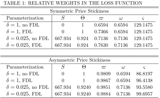
on the policy targets, Table 1 reports the weights of di¤erent stabilization objectives in (18), under
alternative settings. As we shall see in the next section, factor demand linkages have major e¤ects on
the transmission of shocks to the economy. However, their impact on the welfare criterion appears
limited. Analogous considerations apply to consumption goods durability. By contrast, imposing
di¤erent degrees of sectoral price rigidity has considerable in‡uence on the parameterization of the
welfare metric.
Insert Table 1 here
2 1Further details on the linear approximation of this term are available in the technical appendix. Assuming durables
accumulation smoothing as a stabilization objective should help at counteracting the ampli…cation e¤ect of changes in the stock demand of durables on the ‡ow demand of newly produced durable goods. However, as discussed by Erceg and Levin (2006) this term makes a relatively minor contribution to the overall loss. To see this, consider that S de2
t ' d
1 2+ (1 ) (1 !)
e
cd t
2
. As a matter of fact, the …rst term in the square brackets is relatively small, as even large values of are inevitably counteracted by the factor d
1 2 .
2 2Needless to say, eliminating structural asymmetries between sectors and assuming perfectly correlated
shocks would render the two-sector model observationally equivalent to the standard (one sector) New Keynesian model. In this case the loss function would reduce to the familiar benchmark SW0
UH(H)H
2 E0
P1 t=0
t
( +v)yet2+"( )
1 2
t +t.i.p.+O k k
3
4.2 Heterogeneity and Sectoral Stabilization
As the model accounts for several frictions and distortions (e.g., relative price distortions,
price-setting frictions, imperfect labor mobility, inter-sectoral input-output interactions), it is important
to examine how each of them a¤ects sectoral stabilization under the optimal monetary policy. To
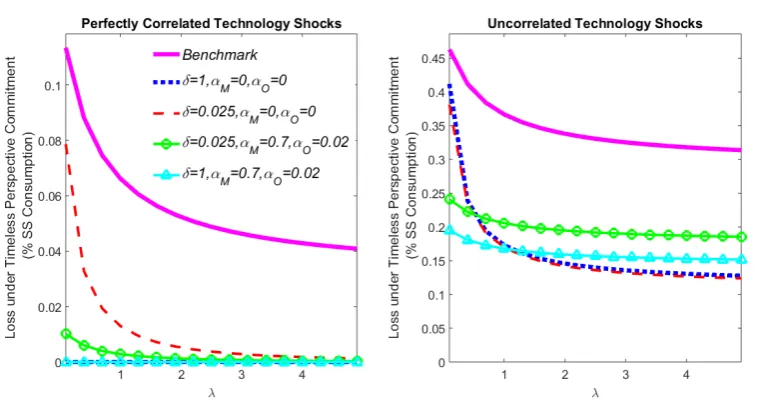
this end, Figure 1 reports the loss of welfare under alternative benchmark models, as a function of
the degree of labor mobility.23 Speci…cally, the upper panels of Figure 1 consider a situation with
symmetric price stickiness, while the remaining panels account for the presence of relatively more
‡exible prices for durables.
Petrella and Santoro (2011) have shown that even under perfect labor mobility (i.e., ! 1) the
central bank may not attain the Pareto optimal allocation consistent with the full stabilization of both
sectors (i.e., manufacturing and services), unless the technology shock bu¤eting one sector equals the
other one, scaled by the ratio between the sectoral income shares of input materials. This condition
is invariant to the presence of goods with di¤erent durability. However, no full stabilization can be
attained in the present setting, unless a rather restrictive set of assumptions are made, as stated by
Proposition 1.
Proposition 1 In the model with sticky prices and perfect labor mobility across sectors, there exists
no monetary policy that can attain the Pareto optimal allocation unless the following condition is
met:24
ztd Odstd
znt Onstn
= Ld
Ln
: (25)
Proof. See Appendix C.
4.2.1 Perfectly Correlated Sectoral Shocks
The left-hand panels of Figure 1 consider situations with perfectly correlated sectoral shocks. As
predicted by Proposition 1 a symmetric production structure always ensures full stabilization under
perfect labor mobility, even in the presence of durability. Moreover, full stabilization is attainable
even at low values of in the presence of no durables (i.e., = 1). Otherwise, durability ampli…es the
loss of welfare in the presence of limited labor mobility, even if the relative price remains at its steady
state level by virtue of zn
t =ztd, 8t.25 It should be noted that, under limited labor mobility, the loss
2 3
We temporarily rule out the oil shock and the sectoral cost-push shocks.
2 4Allowing for imperfect labor mobility would only constrain further the ability of the monetary authority to neutralize
exogenous perturbations.
2 5This situation is close to that considered by Erceg and Levin (2006), as they assume partially correlated sectoral
of welfare is attenuated when input materials are employed by symmetric production technologies, as
compared with the case of M n = M d = 0. The mitigation induced by intermediate goods on the
trade-o¤ is more evident at low values of : the underlying intuition is that in the model with input
materials …rms have the chance to adjust the mix of their production inputs even if labor cannot
move across sectors. This option is a priori ruled out when input materials are not employed in the
production process or they feature asymmetric income shares, in which cases a higher loss of social
welfare obtains.
Insert Figure 1 here
Finally, we should note that the absolute value of the loss is consistently lower in the presence of
more ‡exible prices for durables, as we should expect on a priori grounds. As we shall see in Section
4.2.2, this property carries over to the case of uncorrelated shocks.
4.2.2 Uncorrelated Sectoral Shocks
We now focus on the right-hand panels of Figure 1, where we have assumed uncorrelated technology
disturbances. As we know from Proposition 1 full stabilization can never be attained in this case,
even if the two sectors feature the same production structure and labor can move between sectors so
as to o¤set discrepancies between the nominal wage rates. Nevertheless it is worth noting that, while
higher labor mobility tends to o¤set the welfare discrepancies among di¤erent model economies under
symmetric frequencies of price-setting, asymmetric degrees of price rigidity induce quantitatively
im-portant welfare gaps that seem to be insulated from changes in . In fact, asymmetric price stickiness
exacerbates the relative price distortion, and more so when we introduce factor demand linkages in
the two-sector economy with both durables and non-durables. Furthermore, in the baseline
calibra-tion with M n 6= M d the loss of welfare is substantially higher, as compared with the alternative
scenarios.26
In this setting durability tends to attenuate the loss of welfare, no matter whether input materials
are employed in the same proportion across di¤erent sectors or they are excluded from the set of
production inputs. To provide some intuition on this result we assume, without loss of generality,
= 0 and re-write the Euler equation for durable consumption in a more compact form by applying
2 6In fact, asymmetric production technologies always imply the highest loss of welfare, regardless of the correlation
repeated forward substitution:
UCn t
Qt
=
1
X
j=0
(1 )j jEt UDt+j ; (26)
where UCn
t (UDt) is the marginal utility with respect to non-durable (durable) consumption. Barsky,
House, and Kimball (2007) note that in the case of durables with low depreciation rates, the
right-hand side of (26) is heavily in‡uenced by the marginal utilities of durable service ‡ows in the distant
future. When shocks hitting the economy are temporary, the forward-looking terms do not deviate
from their steady-state values, and so even signi…cant variation in the …rst few terms only have a small
impact on the present value. This means that the present value is close-to-invariant, even in the face
of substantial temporary movements in UDt.
27 Given that the right hand-side of (26) remains fairly
constant, any variation in the relative price instantly impacts on the marginal utility of non-durable
consumption: this is exactly what happens under = 0:025. Assuming uncorrelated technology
disturbances induces substantial volatility in Qt, so thatUCn
t ‡uctuates accordingly, especially in the
case of asymmetric price stickiness. Thus, from a policy-making standpoint stabilizing the relative
price is equivalent to stabilizing non-durable expenditure and vice versa. Otherwise, for ! 1 the
stock-‡ow ratio for durables increases and both UCn
t and UDt vary in the face of movements in Qt,
so that it is impossible for the policy maker to jointly stabilize the marginal utilities of di¤erent
consumption goods and their relative price.28
4.3 Impulse-response Analysis
According to Erceg and Levin (2006) the policy maker faces a particularly severe sectoral stabilization
trade-o¤ in the presence of durables, even under the full commitment optimal policy. In light of the
evidence presented so far, embedding sectoral linkages in a two-sector economy with durable and
non-durable goods has non-negligible normative implications. Therefore, it seems important to isolate the
contribution of factor demand linkages to the transmission of shocks under the optimal policy. To
this end, we compare our baseline setting with a model that neglects the presence of input materials.
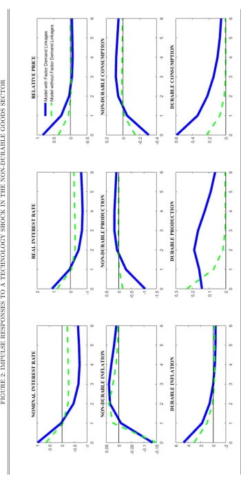
Figure 2 reports equilibrium dynamics following a one-standard-deviation technology shock in the
non-durable goods sector, under di¤erent assumptions about the production structure.29 All variables
2 7
This approximation is equivalent to saying that the demand for durable goods displays an almost in…nite elasticity of intertemporal substitution. Even a small drop in the relative price of durables today relative to tomorrow would cause people to delay their purchases.
2 8Otherwise, the relative price gap can always be closed in the presence of perfectly correlated sectoral shocks and no
durability.
but the interest rate are reported in percentage deviation from their frictionless level. Furthermore,
symmetric nominal rigidity is assumed, with n= d= 0:75.30
Insert Figure 2 here
A positive technology shock in the non-durable goods sector renders the production of these goods
relatively cheaper. However, under sticky prices Ptn is prevented from reaching the level consistent
with prices being set in a frictionless fashion. This determines a drop in the consumption gap of
non-durables. AlsoQtlies above the level that would prevail under ‡exible prices, so that the consumption
gap of durables increases. Therefore, a sector-speci…c technology shock faces the policy maker with
the problem of stabilizing diverging consumption gaps in the two sectors. Faced with divergent
responses of the production gaps in the two sectors, Erceg and Levin (2006) suggest that keeping the
consumption of non-durables at potential requires a "sharp and persistent fall" in the real interest rate.
By contrast, a sharp rise in the policy instrument is required to close the consumption gap of durable
goods. As a result,the nominal rate of interest initially rises to stabilize durables expenditure, and
gradually declines to accommodate the stabilization of non-durable expenditure. In our model with
input materials monetary policy-making features the same type of response, though both the initial
contraction and the subsequent expansion are wider, as compared with the benchmark economy with
no sectoral linkages. In fact, factor demand linkages exacerbate the inter-sectoral stabilization
trade-o¤ that otherwise operates under the traditional demand channel, as indicated by higher reactiveness
of the relative price gap. In turn, the cross-industry ‡ow of input materials ampli…es the response
of non-durable consumption under ‡exible prices, thus inducing a greater drop in their consumption
gap. At the same time, sectoral linkages are responsible for amplifying the response of the durable
consumption gap.
Insert Figure 3 here
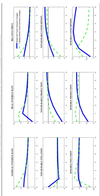
Figure 3 reports equilibrium dynamics following a cost-push shock in the non-durables sector. A
distinctive feature of the model with factor demand linkages is that a rise in the relative price of
non-durables counteracts the de‡ationary e¤ect in the durable sector that otherwise operates through
the conventional demand channel. Concurrently, factor demand linkages are responsible for inducing
a contraction of both the durable and non-durable production gap, while in the benchmark model the
sectoral production gaps display negative co-movement. In light of this, in the presence of sectoral
linkages the central bank pursues a (weakly) contractionary policy, initially accompanied by a negative
3 0As in Strum (2009) we opt for this choice to prevent the central bank from focusing exclusively on the stickier
real rate of interest. Such a policy response is justi…ed by the fact that changes in the relative price
are channeled through the sectoral marginal costs and act as an endogenous attenuator of de‡ationary
pressures in the sector that is not directly hit by the cost-shifter (see (16)).
Insert Figure 4 here
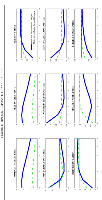
Figure 4 graphs the e¤ects of a drop in the supply of oil. We set the shock so as to induce a one
percentage point increase in the oil price (on impact). As in the face of a sector-speci…c technology
shock, the policy maker is faced with the problem of stabilizing diverging sectoral consumption and
production gaps. In fact, equilibrium dynamics in this case is close to the one we would observe in
the face of a negative technology shock in the non-durable sector, with the central bank opting for a
particularly restrictive policy stance in the model with factor demand linkages. It is also important to
note that combining sectoral in‡ations based on the size of each sector returns an index of general price
in‡ation that is one order of magnitude less volatile than oil price changes. This factor is explicitly
taken into account in the next section, where we build a measure of domestically generated in‡ation
that excludes the price of oil from a measure of general price level, so as avoid that the monetary
policy stance accounts for price movements that are ever too volatile.
5
Alternative Monetary Policy Regimes
This section aims at examining the performance of alternative policy regimes with respect to
policy-making under timeless perspective. We …rst examine a family of interest rate rules that react to
aggregate measures of real activity and in‡ation. We then allow for the possibility that monetary
policy is delegated to a central banker with di¤erent preferences for output and in‡ation stabilization,
as compared with the public, whose welfare criterion is represented by (18). In both cases, we
emphasize the importance of accounting for sectoral heterogeneity and production linkages when
aggregating the sectoral rates of in‡ation into a measure of general price changes.
5.1 Interest Rate Rules
We turn our attention to a family of simple monetary policy rules akin to those examined by Taylor
(1993), Giannoni and Woodford (2003), Schmitt-Grohe and Uribe (2007) and Leith, Moldovan, and
Rossi (2012). A number of empirical contributions (see, among others, Taylor, 1993, Clarida et al.,
2000, Lubik and Schorfeide, 2004) have shown that these policy functions capture, prima facie, the
these rules may mimic the optimal policy, while abstracting from its stringent informational
require-ments.31 As such, our analysis provides us with a direct understanding of how sectoral heterogeneity
a¤ects the implementability of simple instrument rules that target aggregate measures of real
activ-ity and in‡ation. In this respect, …nding the most appropriate in‡ation rate to target is an issue of
concern when dealing with sectoral heterogeneity (see, e.g., Huang and Liu, 2005). We will consider
three alternative measures: (i) aggregate in‡ation, according to which the sectoral in‡ation rates are
aggregated depending on the relative size of each sector; (ii) sticky-price in‡ation, which weighs the
sectoral rates depending on both the relative size and the relative degree of rigidity in price-setting
of each sector; (iii) domestically generated in‡ation, which excludes ‡uctuations in the price of oil –
the only imported good in the economy –from changes in the general price level. The …rst de…nition
may be regarded as a model-consistent counterpart of in‡ation as measured by the growth rate of the
output de‡ator.32 As for sticky-price in‡ation, this is conceived to capture factors that a¤ect relative
price changes, whose importance for sectoral stabilization has been recognized by a number of authors
(see, e.g., Aoki, 2001; Woodford, 2003; Eusepi et al., 2011). Finally, domestically generated in‡ation
allows the central bank to isolate the behavior of general prices without distraction from spikes in
volatile oil prices.33
We examine the welfare properties of a rule that responds to contemporaneous measures of in‡ation
and output gap, as well as a rule characterized by the possibility of adjusting the policy rate with
some gradualism:
it = it+ yyet; (27)
it = it 1+ (1 ) ti+ yyet ; it=
n agg
t ; sticky
t ;
dg t
o
(28)
where
agg
t = { nt + (1 {) dt (29)
sticky
t = $ nt + (1 $) dt (30)
dg
t = 1 {
On n
t On Ot +
1 {
1 Od
d
t Od Ot (31)
3 1
Erceg and Levin (2006) follow an analogous line of reasoning, studying the stabilization properties of targeting rules that, despite the fact the welfare criterion involves sector-speci…c variables, do not consider sector-speci…c output gaps and in‡ation rates.
3 2
It is important to stress that, using the model-consistent de…nition of CPI in‡ation (i.e., CP It = n n t + d
d t), would produce very similar results to those obtained with the output de‡ator.
3 3
where { Yn= Yn+Yd and Ot denotes oil price in‡ation.34 Note that we employ $ as the
weight attached to the rate of in‡ation of non-durables, in line with the factor that balances the
volatility of sectoral in‡ation dynamics in the welfare criterion (18). This convolution of parameters
also depends on the sectoral elasticities of substitution, as in the cost-of-nominal-distortions index
(CONDI) elaborated by Eusepi, Hobijn, and Tambalotti (2011). However, as both elasticities are
calibrated at the same value, sectoral in‡ations are weighted according to the inverse of the slope of
the sector-speci…c New Keynesian Phillips curve.35
We determine the reaction coe¢ cients so that 2 [0;1], 2 [1;5] and y 2 [0;5].36 Thus,
we search for the best combination of the response coe¢ cients to minimize the unconditional welfare
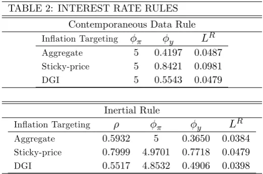
measure in the decentralized equilibrium of the model economy. Table 2 reports these values, together
with the di¤erence between the loss under the optimized rules and that under the optimal policy
benchmark. All losses are computed as a percentage of steady-state consumption.
Insert Table 2 here
Under a contemporaneous data rule consistently hits the upper bound of its support.37 Most
notably, while in a model without input materials it is desirable to set y = 0 when all shocks are at
play,38in the economy under examination it is recommendable to adjust the rate of interest in response
to movements in the output gap, no matter the upper bound we impose on in‡ation responses. This
result is crucially driven by the interplay between durables and inter-sectoral production linkages.
Compared with models where consumers’utility only depends on non-durable consumption, durable
goods introduce additional volatility in the system. Moreover, factor demand linkages magnify the
response of real activity to sectoral cost-shifters, as it has been shown in the previous section. Due
to this additional source of volatility, the policy maker needs to adjust the policy rate in response to
e
yt. To explain why this is possible in the present setting, we need to start from the observation that
increasing the income share of intermediate goods inevitably reduces the slope of the New Keynesian
Phillips curve. This means that the pass-through from the real marginal cost to the rate of in‡ation
is attenuated, relative to the scenario with no input materials. In fact, the real marginal cost of sector
i is a homogeneous function of degree 1 M i 1 ji < 1, with i; j = fn; dg and i 6=j. Such an
3 4
Appendix H reports the analytical steps to derive dgt (see also Buiter, 1998).
3 5In light of this property, the resulting sticky-price in‡ation measure is in line with the in‡ation rate consistent with
the Sticky Price Index published by the Atlanta FED. 3 6The range of variation for and
yis selected so as to retain the property of implementability for the selected policy rule, avoiding to allow for unreasonably high response coe¢ cients to in‡ation and the output gap (see Schmitt-Grohe and Uribe, 2007).
3 7
This is the case no matter the support we consider for the response to the rate of in‡ation. In fact, it is possible to show that raising the upper bound of this value – even to implausibly high values – would marginally improve the loss of social welfare. Additional evidence on this point is available, upon request, from the authors.
3 8
attenuation e¤ect re‡ects the presence of strategic complementarities stemming from the input-output
interactions that take place in each sector. As shown by Basu (1995), this type of interactions have
the potential to turn small price-setting frictions into considerable degrees of real rigidity. From a
policy viewpoint, this ‡attening of the sectoral supply schedules allows the central bank to adjust
the policy rate in response to ‡uctuations in real activity, as variations in the demand of each sector
produce lower e¤ects on prices.
Compared with reacting to either aggregate or domestically generated in‡ation, targeting the
sticky-price rate of in‡ation produces a higher loss of social welfare under both the contemporaneous
data and the inertial rule. This result appears rather surprising, as the literature on optimal
mon-etary policy has posed strong emphasis on the importance of accounting for the relative degree of
price stickiness when aggregating sectoral prices.39 Moreover, a number of central banks are paying
increasing attention to developing measures of general price in‡ation that should account for di¤erent
frequencies of sectoral price adjustment, so as to capture di¤erent aspects of the in‡ation process.40
To dig deeper on this result, we perform an exercise aimed at understanding how the weights attached
to the sectoral rates of in‡ation should optimally be assigned to minimize the loss of social welfare. To
this end, we compute the loss of welfare under two rules: one in which y is set at the value consistent
with aggregate in‡ation targeting, and one in which it equals the value under sticky-price in‡ation
targeting.41 In both cases we set at its upper bound, while varying the weight attached to durable
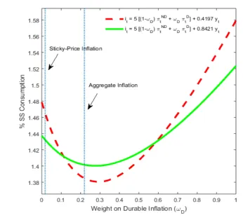
goods in‡ation, !D, over the unit interval.
Insert Figure 5 here
According to Figure 5, under both rules excess loss is minimized at a value of!D that is remarkably
close to the level consistent with targeting aggregate in‡ation. The intuition for this result rests on the
e¤ect exerted by the price of a sectoral good on the cost of producing goods in the other sector. In fact,
even if they are adjusted at shorter time-intervals, durable goods prices inherit considerable persistence
from the price of non-durable goods through factor demand linkages. For analogous reasons, price
stickiness in the non-durable goods sector is partly attenuated due to sectoral complementarities in
price-setting. Therefore, cross-industry interactions in price-setting need to be carefully accounted
for by the central bank when computing measures of (…nal goods) price in‡ation that should keep
3 9
In fact, Woodford (2003) shows that targeting sticky-price in‡ation produces a lower loss of welfare than targeting aggregate in‡ation in a single-sector model with technology shocks. Appendix I supports this prescription for a two-sector model economy without factor demand linkages.
4 0
For instance, Bryan and Meyer (2010) show that sticky prices appear to incorporate expectations about future in‡ation to a greater degree than prices that change on a frequent basis, while ‡exible prices respond more powerfully to economic conditions.
4 1This exercise only considers the two measures of aggregate price changes that can be retrieved as a weighted averages
track of changes in the relative price. In the speci…c setting under examination, the measure of
sticky-price in‡ation that is consistent with the welfare-theoretic function only accounts for intrinsic
in‡ation persistence, while disregarding inter-sectoral input-output interactions as a source of extrinsic
persistence. As a result, even if the durable goods sector features a higher frequency of price-setting
(see, e.g., Bils and Klenow, 2004b and Nakamura and Steinsson, 2008a), sticky-price in‡ation targeting
attaches "too much" importance to non-durable goods in‡ation. This fact is indirectly con…rmed by
Bouakez, Cardia, and Ruge-Murcia (2014), who estimate sectoral Calvo parameters in line with the
results of Nakamura and Steinsson (2008a), implying that available non-structural estimates only
capture intrinsic in‡ation persistence at the sectoral level, while disregarding extrinsic persistence
inherited through production costs and, in turn, input materials.
5.2 Delegation
There are various reasons why monetary policy in practice might depart from the minimization of a
rather convoluted welfare metric, such as (18). For instance, various parameters and components of
the loss function might not be known with certainty and/or the public may opt for delegating monetary
policy to an independent central banker, whose preferences for alternative stabilization objectives di¤er
from those of the public (see, e.g., Rogo¤, 1985). The advantages of a simple mandate are evident in
terms of communication and accountability (see Nunes et al., 2015). Under these circumstances, the
policy rule would depend on the objective function e¤ectively faced by the policy maker. The next
step in the analysis aims at understanding which of the in‡ation rates (29)-(31) should be accounted
for by a policy maker whose welfare criterion only weights ‡uctuations in the output gap against those
in a given measure of general price in‡ation, according with the following welfare function:
LDt =E0
1
X
t=0
th i t
2
+'y(eyt)2
i
: (32)
To this end, we assume that the weight attached to output stabilization, 'y, may vary over a …nite
support, with the weight attached to the quadratic in‡ation term set to one. Concurrently, the loss
of welfare welfare is evaluated through the model-consistent metric, (18).
Insert Figure 6 here
As indicated by Figure 6 attaching a small, yet non zero, weight to output stabilization achieves
the lowest welfare loss. Furthermore, note that sticky-price in‡ation targeting dominates aggregate
in‡ation targeting at'y 0. This can be explained upon examining the weights attached to di¤erent
central bank to pursue a strongly anti-in‡ationary policy, with the weights attached to the quadratic
terms of sectoral in‡ations depending on the relative degree of price rigidity and no concern for
sectoral in‡ation co-movement.42 This feature is captured by the exercise portrayed in Figure 6: at
low values of 'y the loss of the delegated central banker comes closer to mimic (18) by considering a
measure of sticky-price in‡ation, which attaches little or no weight to the cross-term involving sectoral
in‡ations. By contrast, when the policy maker receives a dual mandate that stresses both in‡ation
and output stabilization, weighting sectoral in‡ations based on the size of each sector is preferable,
and more so at intermediate values of 'y.43 Once again, the intuition for this result depends on the
‘e¤ective’degree of sectoral price stickiness and how this is weighed by alternative indices of general
price in‡ation. In fact, balancing sticky-price in‡ation volatility with output gap volatility does not
allow the central banker to tackle the intra-sectoral trade-o¤ in the durable goods. This is because,
by virtue of 'y > 0, the dual mandate implicitly attributes a sizeable weight to the stabilization of
durable goods production, while durable goods in‡ation is close to be neglected, despite their cost
of production inherits a certain degree of extrinsic persistence through the cost of input materials
supplied by the non-durable goods sector.
Finally, it is worth noting that delegating monetary policy to a central banker concerned with
stabilizing domestically generated in‡ation results into a higher loss of welfare, as compared with
tar-geting either aggregate or sticky-price in‡ation. This is because the trade-o¤ captured by a tartar-geting
rule involving domestically generated in‡ation and output volatility compares, de facto, a measure
of in‡ation that is insulated from swings in the price of oil with a measure aggregate real activity
that is instead a¤ected by oil price dynamics. Not surprisingly, such a policy setting turns out to be
suboptimal with respect to both alternatives.
6
Conclusions
We have presented a two-sector New Keynesian economy that features sectoral heterogeneity along
three main dimensions: price stickiness, consumption goods durability, inter-sectoral trade of input
materials. Such distinctive traits of modern industrialized economies display non-trivial interactions
that limit both inter-sectoral and intra-sectoral stabilization. In this context we examine the potential
of some simple interest-rate feedback rules to mimic the optimal policy under timeless perspective
com-mitment. A clear advantage of these policy functions is to abstract from the stringent informational
4 2Table 1 highlights how the weight on the quadratic terms involving the sectoral rates of in‡ation is substantially
larger than the overall weight attached to the quadratic terms involving real activity.
requirements implied by the welfare-theoretic loss function, which involves sector-speci…c variables.
To this end, we assume that the policy rate is adjusted in response to aggregate measures of real
activity and in‡ation. Asymmetric degrees of price rigidity and inter-sectoral production linkages do
matter when it comes to aggregating sectoral in‡ation rates into an overall index of price in‡ation.
Even if non-durable goods prices are assumed to be relatively stickier, durable goods in‡ation inherits
considerable extrinsic persistence through the intermediate input channel.
The present work carries a key implication for the computation of appriopriate measures of
aggre-gate in‡ation. A policy maker that neglects sectoral production linkages may incur in a severe bias
when trying to compute broad measures of in‡ation that should keep track of relative price changes,
aggregating sectoral in‡ations based on the relative size of each sector and the relative degree of price
rigidity. In fact, the available estimates of sectoral price rigidity only account for a measure of notional
stickiness in price-setting, while disregarding inherited stickiness through production costs, which are
in turn a¤ected by the price of input materals.
References
Aoki, K. (2001): “Optimal Monetary Policy Responses to Relative Price Changes,”Journal of
Monetary Economics, 48, 55–80.
Barsky, R. B., C. L. House, and M. S. Kimball (2007): “Sticky-Price Models and Durable
Goods,”American Economic Review, 97(3), 984–998.
Basu, S. (1995): “Intermediate Goods and Business Cycles: Implications for Productivity and
Wel-fare,”American Economic Review, 85(3), 512–31.
Bernanke, B. S. (1985): “Adjustment costs, durables, and aggregate consumption,”Journal of
Monetary Economics, 15(1), 41–68.
Bils, M.,andP. J. Klenow(2004a): “Some Evidence on the Importance of Sticky Prices,”Journal
of Political Economy, 112(5), 947–985.
(2004b): “Some Evidence on the Importance of Sticky Prices,”Journal of Political Economy,
112(5), 947–985.
Blanchard, O. J., andJ. Galí(2007): “The Macroeconomic E¤ects of Oil Price Shocks: Why are
the 2000s so di¤erent from the 1970s?,” in International Dimensions of Monetary Policy, NBER