Using linear mixed model and dummy variable  model approaches to construct compatible single tree biomass equations at different scales – A case study for Masson pine in Southern China

JOURNAL OF FOREST SCIENCE, 58, 2012 (3): 101–115

Since forest ecosystems play irreplaceable roles in regulating global carbon balance and mitigating global climate change, forest biomass monitoring is becoming more important (Tomppo et al. 2010). It is fundamental for monitoring and assessment of national forest biomass to develop generalized single-tree biomass models suitable for large-scale forest biomass estimation. In recent years, many re-searchers have attempted to construct generalized single-tree biomass models applying them to for-est biomass for-estimation on a regional, national, even global level. Hansen (2002) compared four differ-ent methods currdiffer-ently being used by the Forest

In-ventory and Analysis (FIA) program of the USDA Forest Service to estimate the gross volume and total biomass, and showed that these four methods produced similar results, but large differences exist-ed for specific species and diameters, so the author recommended that FIA would develop a nationally consistent method for estimating volume and bio-mass. Chojnacky (2002) and Jenkins et al. (2003) developed a set of national-scale generalized above-ground biomass equations for main tree species in the USA. In the countries such as France, Iceland, Finland and Mexico, the tree biomass or volume equations of main species were also constructed in

Supported by the Ministry of Science and Technology, Projects No. 31070485, No. 31170588, and No. 2006BAD23B02.

Using linear mixed model and dummy variable model

approaches to construct compatible single-tree biomass

equations at different scales – A case study for Masson

pine in Southern China

L.Y. Fu

_{, W.S. Zeng}

_{, S.Z. Tang}

_{, R.P. Sharma}

_{, H.K. Li}

1_{Research Institute of Forest Resource Information Techniques, Chinese Academy of Forestry,}

Beijing, China

2_{Academy of Forest Inventory and Planning, State Forestry Administration, Beijing, China} 3_{Department of Ecology and Natural Resource Management, Norwegian University of Life}

Sciences, Ås, Norway

ABSTRACT: The estimation of forest biomass is important for practical issues and scientific purposes in forestry. The estimation of forest biomass on a large-scale level would be merely possible with the application of generalized single-tree biomass models. The aboveground biomass data on Masson pine (Pinus massoniana) from nine provinces in southern China were used to develop generalized single-tree biomass models using both linear mixed model and dummy variable model methods. An allometric function requiring only diameter at breast height was used as a base model for this purpose. The results showed that the aboveground biomass estimates of individual trees with identical diameters were different among the forest origins (natural and planted) and geographic regions (provinces). The linear mixed model with random effect parameters and dummy model with site-specific (local) parameters showed better fit and prediction performance than the population average model. The linear mixed model appears more flexible than the dummy variable model for the construction of generalized single-tree biomass models or compatible biomass models at different scales. The linear mixed model method can also be applied to develop other types of generalized single-tree models such as basal area growth and volume models.

recent years (Snorrason, Einarsson 2006; Val-let et al. 2006; Repola et al. 2007; Návar 2009). In Europe, the generalized allometric volume and biomass equations for five tree species were de-veloped by Muukkonen (2007). In addition, from the comparison of prediction errors of local, gen-eralized regional and national tree biomass and volume equations of 10 species for the boreal for-est region of wfor-est-central Canada, Case and Hall (2008) found that there was a concomitant increase in prediction error from increasing levels of equa-tion generalizaequa-tion. Now, the development of gen-eralized national single-tree biomass equations is actively propelled in China. The practical demand for regional and provincial forest biomass estima-tion should be taken into consideraestima-tion when de-veloping national-scale generalized biomass equa-tions. How to construct both national and regional or provincial generalized models, when the condi-tions are allowed, and make them compatible with each other is a crucial problem.

The concept of compatibility is well known, but the exact meanings under different situations are not always the same. In this paper, the compatibility means that the biomass models at different scales are compatible with each other. That is, the large-scale sum of estimates from small-large-scale models is the same as the estimate from the large-scale mod-el. The objective of the study is to develop compat-ible single-tree biomass equations at both national and regional or provincial scales, and linear mixed model and dummy variable model methods to pro-vide possible approaches for solving this problem.

The mixed-effects model approach is a statistical technique generating improvements in parameter estimation that has been used in many fields of study for nearly twenty years. In forestry, studies using mixed-effects model approaches are relative-ly recent. Lappi and Bailey (1988) described the use of nonlinear mixed-effects growth curve based on the Richards model, which was fitted to predict dominant and codominant tree height, both at the plot level and at the individual tree level. Gregoire et al. (1995) studied linear mixed-effects modelling of the covariance among repeated measurements with random plot effects. Zhang and Borders (2004) used the mixed-effects modelling method to estimate tree compartment biomass for inten-sively managed loblolly pine (Pinus taeda) plan-tations in the Lower Coastal Plain and Piedmont of Georgia in the USA. Fehrmann et al. (2008) employed the mixed-effects modelling method to establish single-tree biomass equations for Norway spruce (Picea abies) and Scots pine (Pinus

sylves-tris), and compared it with the k-nearest neighbour approach for biomass estimation. Studies such as linear mixed model of aerial photo crown width and ground diameter (Lang 2008), individual basal area growth model using a multi-level linear mixed model with repeated measurements (Lei et al. 2009), and modelling dominant height for Chinese fir (Cunninghamia lanceolata) plantation using a nonlinear mixed-effects modelling approach (Li, Zhang 2010) can be cited as recent publications of mixed-effects models in forestry in China.

In regression analysis, a dummy variable (also known as indicator variable) takes the values 0, 1 or –1 to indicate the absence or presence of some categorical effect. Dummy variable processing is a commonly used method to deal with indica-tor or categorical variables, which are involved in all quantitative methods (Tang, Li 2002; Li et al. 2006; Tang et al. 2008). In regression analyses and modelling studies, dummy variable models are usu-ally applied (Li, Hong 1997; Li et al. 2008).

For the two kinds of subject-specific model-ling methods, dummy variable model and mixed-effects model, the choice of which one should be used has been a hot debate in biometrics and sta-tistics (Wang et al. 2008). Wang et al. (2008) made an empirical comparison of the two approaches to dominant height modelling, and concluded that the two kinds of methods were appropriate to con-struct models with specific or local parameters, and produced almost the same outcomes; in terms of height growth description, the dummy variable method was preferred, and in terms of height pre-diction, the mixed-effects modelling method might be appropriate.

MATERIAL And METHOdS

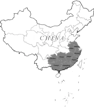
The fit data of 150 sample trees used in this study were the aboveground biomass measurements of Masson pine in Southern China, which were ob-tained from destructive sampling in 2009. The sam-ple trees were located in Jiangsu, Zhejiang, Anhui, Fujian, Jiangxi, Hunan, Guangdong, and Guizhou provinces and Guangxi autonomous region (20 to 35°N, 102‒123°E, Fig. 1). The number of sample trees was approximately distributed by the propor-tion to the stocking volume of Masson pine forests in the nine provinces or autonomous region, and the origins of forests were also taken into account. Among them, a total of 77 trees were from natural forests and 73 trees from plantations. The sample trees were distributed equably in the ten diameter classes of 2, 4, 6, 8, 12, 16, 20, 26, 32 +, and more than 38 cm, i.e. 15 trees for each diameter class ex-cept for 26 cm and 32 cm classes, in which there were 14 and 16 trees, respectively. In addition, the sample trees in each diameter class were distrib-uted by 3–5 height classes as evenly as possible, i.e. 3–5 trees for each height classes. Thus, the sample trees were representative in the large-scale region.

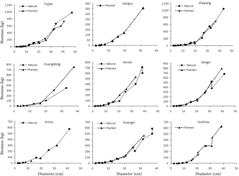
Diameter at breast height of each sample tree was measured in the field. After the tree was felled, the total length of tree (tree height) and length of live crown were also measured. The fresh weights of stem wood, stem bark, branches, and foliage were measured, and subsamples were selected and weighed in the field. After taken to the laboratory, all subsamples were oven dried at 85°C until a con-stant weight was reached. According to the ratio of dry weight to fresh weight, each compartment mass could be computed and the aboveground bio-mass of the tree was obtained by summation. The distribution of sample trees by origins, provinces, and diameter classes is listed in Table 1, and the re-lations between biomass and diameter for different origins in the nine provinces are shown in Fig. 2.

In addition, two sets of aboveground biomass data from Masson pine plantations were used for validation: (i) data from 50 sample trees collected by the South Team of the National Biomass Model-ling Program in 1997 from the Lizhai Forest Farm of Dexing county in Jiangxi province; and (ii) data from 295 sample trees collected in 2007 from Guizhou province for establishment of forestry tables for Masson pine, which were located in the

Fig. 2. The relationship between biomass and diameter for different origins in the nine provinces

growing regions of the species and representative of the population.

Base model

In general, individual tree biomass includes sev-eral compartments such as stem wood, stem bark, branches, foliage, and roots (fine roots less than 2 mm in diameter not to be included). However, the total biomass, especially the aboveground bi-omass, was mainly concerned for large-scale for-est biomass monitoring (FAO 2006; Muukkonen 2007; Tomppo et al. 2010). The allometric biomass equation based on one single variable D (diameter at breast height) was widely used due to predic-tion precisions (e.g. Ter-Mikaelian, Korzukhin 1997; Jenkins et al. 2003; Muukkonen 2007; Ná-var 2009; Fu et al. 2011). We also used the follow-ing allometric function as a base model to construct different biomass equations in this study:

M = aDb_{(1 + ζ) (1)}

where:

M – aboveground biomass,

a, b – parameters, ζ – relative error term.

Model (1) becomes to the following linear form by logarithmic transformation:

y = a₀ + bx + ς (2)

where:

y – ln M, x – ln D, a₀ – ln a,

ς – ln (1 + ζ).

Given to the fitting result of model (2), the bio-mass estimate can be obtained from the following equation:

M^ = exp(a₀ + bx) (3)

However, because some bias resulted from the logarithmic transformation, bias correction was

Diameter (cm) Diameter (cm) Diameter (cm)

Bioma

ss (kg)

Bioma

ss (kg)

Bioma

necessary, and the commonly used correction fac-tor was exp(S2_{/2) (Baskerville 1972;}

Flewel-ling, Pienaar 1981). Then, the corrected estimate of biomass is as follows:

M^ = exp(a₀ + S2_/2)Db ₍₄₎

In addition, viewing from the practical use, the ratio estimator for bias correction in logarithmic regressions presented by Snowdon (1991) could be applied, which might permit the total mean bias to be zero.

However, the aboveground biomass of a tree is impacted not only by diameter but also by other factors, such as origin of the tree and the grow-ing region. In this paper, the one-variable model (2) with two general parameters (also known as global or fixed parameters) was called the popula-tion average (PA) model. Then, the dummy vari-able model and the mixed model involving effects of different tree origins and growing regions were taken into account. Considering that the allomet-ric coefficient b in model (2) is almost stable, some researchers even suggested to use a constant value (West et al. 1999; Chojnacky 2002), therefore, only the impact of local or random effects of differ-ent origins and regions on parameter a₀ was stud-ied in this paper. Forest origins are classifstud-ied into 2 types: natural and planted, whose codes are 1 and 2, and numbers of sample trees are 77 and 73, re-spectively. Geographic regions involve 9 provinces or autonomous region, and the numbers of sample trees for each region are very different (Table 1 and Fig. 2). Based on an overall consideration of water, heat and the number of sample trees, the geograph-ic regions are classified into 3 types: eastern region (Jiangsu, Zhejiang, Fujian), south-central region (Jiangxi, Hunan, Guangdong), and north-western region (Anhui, Guizhou, Guangxi), whose codes are 1, 2, and 3, respectively, and the number of sam-ple trees for each type is 50.

dummy variable model

The general form of dummy variable model based on model (2) is as follows:

y = a₀ + ∑a_iz_i + bx + ς (5)

where:

z_i – dummy variable,

a_i – corresponding specific or local parameter Other symbols are the same as in model (2).

To make a difference, the parameters in dummy model corresponding to those in PA model are called general or global parameters. For obviously understanding the compatibility of different scale models and simply comparing with the mixed models, the processing of dummy variables would meet ∑a_i= 0. Under the restricted condition, only

i–1 special parameters need to be estimated, the last one can be derived from the others.

Because of involving two origins (natural and planted) and three regions, dummy variable pro-cessing may include four different situations. The dummy variable combinations of each situation are listed in Table 2.

Because model (5) is the typical linear equa-tion, the ordinary least-squares (OLS) method can be used to estimate the parameters. It should be pointed out that the model under the 4th _situation

is the full model, based on which we would have nested models that apply at different scales, just like the models under the 1st _{and 2}nd _{situations and}

the PA model.

Linear mixed model

The general form of linear mixed-effects model is as follows (SAS 1999; Tang, Li 2002; Tang et al. 2008):

y = x β + z u + e (6)

n×1 n×p p×1 n×q q×1 n×1

where:

y – dependent variable, β – fixed parameter,

u – random parameter,

x – designed matrix of fixed parameters,

z – designed matrix of random parameters,

e – error matrix.

The mixed model corresponding to model (5) is expressed as follows:

y = a₀ + ∑u_iz_i + bx + ς (7)

where:

the expected values of random parameters u_i – zero, and they are independent of each other.

That is E(u_i) = 0, and cov(u_i, u_j) = 0 for i ≠ j.

Contrasting to the four situations for dummy variable processing above, the followings are taken into account in mixed models:

(ii) Growing region is considered as random variable;

(iii) Both tree origin and growing region are con-sidered as random variables;

(iv) The combinations (interactions) of origin and region are considered as random variables. The linear mixed-effects model (6) or model (7) were fitted using the “Linear Mixed Model” func-tion of “Statistic Analysis” mode in ForStat2.1, in which the method of restricted maximum likeli-hood (REML) was implemented for parameter es-timation (Tang et al. 2008).

Model evaluation

To compare and evaluate the dummy variable model and linear mixed model, three fit statistics were used, which were determination coefficient (R2_{), sum of square errors (SSE), and mean square}

errors (S2_{). They were calculated by the following}

equations:

R2 _{= 1 –}

∑

i – y^ i)2/

∑

SSE =

∑

S2 _{= SSE (n – p) (10)}

where:

y_i, ^ y_i – observed and estimated values of the ith _sample

tree,

y

– _{– arithmetic mean of all observed values,}

n – number of sample trees,

p – number of parameters.

The difference between dummy variable model (or mixed model) and PA model was tested by us-ing an F-statistic, which was computed and com-pared with the critical F value to determine if they were significantly different. The F-statistic was cal-culated as follows (Meng et al. 2008):

(SSE_PA – SSE_DM)/(df_PA – df_DM)

F = –––––––––––––––––––––––– (11) SSEDM/dfDM

where:

SSE_PA, SSE_DM – sums of square errors of the PA model and dummy variable model (or mixed model), respectively,

df_PA, df_DM – the degrees of freedom of the PA model and dummy variable model (or mixed model), respectively.

RESULTS

Using the aboveground biomass data on 150 sam-ple trees of Masson pine from 9 provinces or au-tonomous region in Southern China, the PA model (2) was fitted by the OLS method at first; then the dummy variable model (5) and linear mixed-effects model (7) under the afore-mentioned four situations were fitted through the ForStat2.1 software (Tang et al. 2008).

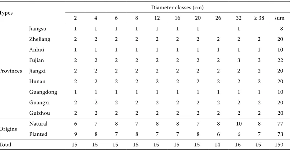
Table 1. The distribution of sample trees of Masson pine in Southern China by origins, provinces, and diameter classes

Types Diameter classes (cm)

2 4 6 8 12 16 20 26 32 ≥ 38 sum

Provinces

Jiangsu 1 1 1 1 1 1 1 1 8

Zhejiang 2 2 2 2 2 2 2 2 2 2 20

Anhui 1 1 1 1 1 1 1 1 1 1 10

Fujian 2 2 2 2 2 2 2 2 3 3 22

Jiangxi 2 2 2 2 2 2 2 2 2 2 20

Hunan 2 2 2 2 2 2 2 2 2 2 20

Guangdong 1 1 1 1 1 1 1 1 1 1 10

Guangxi 2 2 2 2 2 2 2 2 2 2 20

Guizhou 2 2 2 2 2 2 2 2 2 2 20

Origins Natural 6 7 8 7 8 8 7 8 10 8 77

Planted 9 8 7 8 7 7 8 6 6 7 73

PA model

The PA model of aboveground biomass of Mas-son pine in southern China by logarithmic trans-formation is as follows:

y = –2.2368 + 2.3724x (R2 _{= 0.9865, SSE = 9.7095,}

S2 _{= 0.0656, F = 10,795.94, P = 0.0000) (12)}

where:

y = ln M,

x = ln D,

F value = statistic for significance,

P-value = significance level,

t-values of the parameters a₀ and b are – 37.31 and 103.90, respectively.

Table 2. The dummy variable combinations for four different situations

Situations Considered factors Combinations z₁ z₂ z₃ z₁₁ z₁₂ z₁₃ z₂₁ z₂₂

1 origin nature 1

planted –1

2 region

eastern 1 0

south-central 0 1

north-western –1 –1

3 origin + region

nature + eastern 1 1 0 nature + south-central 1 0 1 nature + north-western 1 –1 –1 planted + eastern –1 1 0 planted + south-central –1 0 1 planted + north-western –1 –1 –1

4 origin × region

nature × eastern 1 0 0 0 0

nature × south-central 0 1 0 0 0

nature × north-western 0 0 1 0 0

planted × eastern 0 0 0 1 0

planted × south-central 0 0 0 0 1

planted × north-western –1 –1 –1 –1 –1 z₁, z₂, z₃, z₁₁, z₁₂, z₁₃, z₂₁, z₂₂ – dummy variables

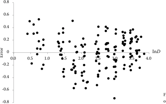
Fig. 3. Distribution of residual errors of the PA model (12)

-0.8 -0.6 -0.4 -0.2 0 0.2 0.4 0.6 0.8

0.0 0.5 1.0 1.5 2.0 2.5 3.0 3.5 4.0

Er

ror

lnD

The distribution of residual errors of the PA mod-el (12) is shown in Fig. 3.

The aboveground biomass equation correspond-ing to model (4) is as follows:

M^ =exp(–2.2368 + 0.0328) D2.3724

where:

M^ – predicted value of aboveground biomass,

D – diameter of the tree.

This is the generalized biomass model to be used for national forest biomass estimation.

dummy variable model

The fitting results of dummy variable models un-der the four situations above (named as models 1, 2, 3, and 4 in order) are listed in Table 3.

It is shown in Table 3 that the differences among the estimates of specific parameters in models 1, 2 and 3 are rather small because the effects are inde-pendent in the models; but the estimates of specific parameters in model 4 are very different from those in the other three models, because the interactions of tree origin and growing region are considered here.

From F-test of the four dummy variable models and the PA model, the F-values calculated by equa-tion (11) were 2.30, 1.68, 1.82 and 2.41, respective-ly. Only model 4 was significantly different from the PA model at a 0.05 level, and the other three models were not significantly different from the PA model at 0.05 and 0.10 levels.

Based on dummy model 4, we can obtain the fol-lowing nested models contrasting to the PA model, model 1 and model 2:

PA model:

M^ =exp(–2.2153 + 0.0313) D2.3653

Model 1 for the natural forest:

M^ =exp(–2.2153 + 0.0299 + 0.0313) D2.3653

Model 1 for the planted forest:

M^ =exp(–2.2153 – 0.0299 + 0.0313) D2.3653

Model 2 for region 1:

M^ =exp(–2.2153 + 0.0369 + 0.0313) D2.3653

Model 2 for region 2:

M^ =exp(–2.2153 + 0.0132 + 0.0313) D2.3653

Model 2 for region 3:

M^ =exp(–2.2153 – 0.0501 + 0.0313) D2.3653

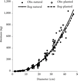
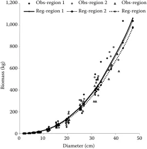
The regression curves of dummy models for dif-ferent origins (model 1 above) and for difdif-ferent re-gions (model 2 above) are shown in Figs. 4 and 5.

Linear mixed model

The fitting results of linear mixed-effects mod-els under the afore-mentioned four situations are listed in Table 4. In addition, from F-test of the four mixed models and the PA model, the F-values cal-culated by equation (11) were 2.31, 2.35, 2.27 and 3.36, respectively. Model 4 was significantly differ-ent from the PA model at a 0.01 level, and mod-els 2 and 3 were significantly different from the PA model at a 0.10 level, but mixed model 1 was not significantly different from the PA model, just like dummy variable model 1.

Based on mixed model 4, similarly like the dum-my model, we can obtain the following nested models contrasting to the PA model, model 1 and model 2:

PA model:

M^ =exp(–2.2243 + 0.0313) D2.3683

Model 1 for the natural forest:

M^ =exp(–2.2243 + 0.0179 + 0.0313) D2.3683

Model 1 for the planted forest:

M^ =exp(–2.2243 – 0.0179 + 0.0313) D2.3683

Model 2 for region 1:

M^ =exp(–2.2243 + 0.0225 + 0.0313) D2.3683

Model 2 for region 2:

M^ =exp(–2.2243 + 0.0069 + 0.0313) D2.3683

Model 2 for region 3:

M^ =exp(–2.2243 – 0.0294 + 0.0313) D2.3683

dISCUSSIOn

Comparison of the two kinds of models

It is shown in Tables 3 and 4 that the special and random parameters of natural type are positive whereas those of planted type are negative (two effects cancel each other out). This indicates that the aboveground biomass of a tree in natural for-est is larger than that in planted forfor-est when the tree diameter is the same, but the differences are not statistically significant. As for region types, the aboveground biomass of a tree with the same diam-eter gradually decreases from the eastern region to south-central and north-western regions, but the differences are not statistically significant either. The impacts of tree origin and growing region re-flected in the mixed models showed the same pat-tern as in the dummy models. In terms of the three fit statistics (R2_{, SEE, and S}2_{), there was no large}

dummy model and mixed model resulted from the fact that the dummy model had a lower degree of freedom than the corresponding mixed model in which the specific parameters were assumed to follow a normal distribution, and the number of independent parameters was decreased. In fact, in terms of other two criteria independent of the degree of freedom, R2 _{and SEE, the dummy model}

was slightly better than the mixed model, which was consistent with the conclusion presented by Wang et al. (2008).

We know that in dummy model the specific pa-rameters are usually processed and estimated as-suming the responsible value of one type (usu-ally the type with the smallest expected value) to be zero. In this study, the commonly used values (1, 0) were instead of (1, –1) in dummy model,

which could assure the sum of responsible values of all types to be zero, just like in mixed model. For example, in dummy model 1, the estimates of specific parameters for natural and planted forests were 0.0317 and –0.0317, respectively, and in mixed model 1 the estimates of random parameters were 0.0179 and –0.0179, respectively. Although the same pattern was shown, i.e. the responsible value of natural forest was higher than that of planted for-est, the sizes were different: the difference between the two parameters in dummy model was 0.0634, but the difference in mixed model was only 0.0358. The specific parameters of dummy model and the random parameters of mixed model in models 2–4 showed the same pattern. That means the dif-ference among specific types reflected in mixed model is smaller than that in dummy model, which

Fig. 4. The regression curves of dummy mo-del 1 for different origins

1,000

1,200 _{Obs-Natural Obs-Planted}

Reg-Natural Reg-Planted

400 600 800 1,000

0 200 400

0 10 20 30 40 50

Diameter (cm) 0

0 10 20 30 40 50

Diameter (cm)

0 10 20 30 40 50

Diameter (cm) Obs-natural

Reg-natural

Obs-planted Reg-planted 1,200

1,000

800

600

400

200

0

Bioma

ss (kg)

Table 3. The results of dummy variable model (5)

Dummy models

General

parameters Specific parameters Fit statistics

a₀ b a₁ a₂ a₃ a₄ a₅ a₆ F-value P-value R2 _{SEE S}2

is consistent with the conclusion presented after a comprehensive comparison of the two kinds of models by Wang et al. (2008). Wang et al. (2008) stated that if the variance of random effects were very large relative to the error variance, the random parameter estimates would be very close to what they would be if they were regarded as fixed pa-rameters; and if the random effects showed a very small variance, the random parameter estimates would be very close to zero, i.e. the mixed model would be very close to the PA model. Thus, they claimed that the mixed model might be regarded as a compromise between the dummy model in which the specific parameters are fixed and the PA model in which the specific parameter are zero.

In order to show the differences among dummy model, mixed model and PA model, and to dem-onstrate the compatibility of the models at differ-ent scales, the results of aboveground biomass

es-timation (logarithmic transformation) from the PA model, dummy and mixed models under the four situations mentioned above are listed in Table 5, where model 0 means the PA model (12).

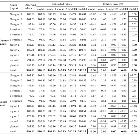
It is shown in Table 5 that though the total es-timate of the PA model is unbiased (total relative error is equal to 0), the estimates for different ori-gins, regions, and their combinations have relative errors lower than ± 3%; and the dummy and mixed models under the four situations can decrease the errors of estimates for various types, among which models 1 and 2 improve slightly, and models 3 and 4 improve more; and furthermore, model 4 con-sidering the interactions of origins and regions is better than model 3 considering the effects of ori-gins and regions independently. Dummy model 4 is equivalent to six models with specific parameters for the six combinations of origins and regions, and the specific parameters are all regarded as fixed

pa-Table 4. The results of linear mixed model (7)

Mixed models

Fixed parameters Random parameters Random effects analyses Fit statistics a₀ b u₁ u₂ u₃ u₄ u₅ u₆ F-value significant R2 _{SEE S}2

Model 1 –2.2327 2.3706 0.0179 –0.0179 1.5764 – 0.9867 9.5594 0.0650 Model 2 –2.2367 2.3724 0.0165 0.0041 –0.0206 1.3273 – 0.9867 9.5565 0.0650 Model 3 –2.2328 2.3706 0.0171 –0.0171 0.0159 0.0030 –0.0189 0.8572/1.2279 – 0.9869 9.4170 0.0645 Model 4 –2.2243 2.3683 0.0642 –0.0180 0.0075 –0.0191 0.0318 –0.0664 1.4668 – 0.9874 9.0785 0.0626

Fig. 5. The regression curves of dummy model 2 for different regions

0 200 400 600 800 1,000 1,200

0 10 20 30 40 50 Obs-Region1 Obs-Region2 Obs-Region3 Reg-Region1 Reg-Region2 Reg-Region3

0

0 10 20 30 40 50 Diameter (cm)

0 10 20 30 40 50 Diameter (cm)

Obs-region 2 Reg-region 2 Obs-region 1

Reg-region 1

Obs-region 3 Reg-region 3 1,200

1,000

800

600

400

200

0

Bioma

rameters, thus the total estimates for six types and the sums by origin or region have no errors (the relative errors of about ± 0.01% in Table 4 resulted from the computing precision, they are equal to zero theoretically). However, in mixed model 4, the impacts of the six combinations of origins and re-gions are treated as random effects, and the specific parameters are regarded as random parameters, thus the total estimates for six types and the sums by origin or region still have about ± 1% relative er-rors, where the total estimate for the type of plant-ed-region 3 has the largest relative error 1.27%.

Moreover, whether it is dummy model or mixed model, the sums of estimates by origin, region or their combinations are all equal to the total

esti-mate of the PA model. That is to say that the nation-al sums of estimates of region-specific models are the same as the national estimate of the PA model. Thus, the PA model and the dummy and mixed models at different scales are compatible.

Analysis and validation of the models

For the dummy model and mixed model, the choice of which one should be used has been a hot debate in biometrics and statistics (Wang et al. 2008). Viewing from the practical application, the choice can be made depending on the number of subjects/types and the number of samples per type:

Table 5. The estimation results of the models at different scales for fit data

Scales

(types) Observed values

Estimated values Relative error (%)

model 0 model 1 model 2 model 3 model 4 model 0 model 1 model 2 model 3 model 4

Dummy model

N-region 1 105.82 103.04 103.79 104.06 104.79 105.81 –2.62 –1.91 –1.66 –0.96 0.00 N-region 2 104.03 104.80 105.70 105.10 105.83 104.03 0.74 1.60 1.03 1.73 0.00 N-region 3 85.14 84.80 85.50 83.62 84.37 85.15 –0.41 0.42 –1.79 –0.91 0.01 P-region 1 76.40 77.14 76.34 78.16 77.42 76.40 0.97 –0.07 2.31 1.34 0.01 P-region 2 76.72 75.44 74.76 75.65 74.92 76.72 –1.67 –2.56 –1.39 –2.35 0.00 P-region 3 92.02 94.92 94.04 93.54 92.80 92.01 3.15 2.19 1.65 0.84 –0.01 region 1 182.21 180.17 180.13 182.21 182.21 182.21 –1.12 –1.14 0.00 0.00 0.00 region 2 180.76 180.25 180.46 180.75 180.75 180.75 –0.28 –0.16 0.00 0.00 0.00 region 3 177.16 179.71 179.54 177.16 177.16 177.16 1.44 1.34 0.00 0.00 0.00 natural 294.98 292.64 294.99 292.78 294.99 294.99 –0.80 0.00 –0.75 0.00 0.00 planted 245.15 247.49 245.14 247.35 245.14 245.14 0.96 0.00 0.90 0.00 0.00 total 540.13 540.13 540.13 540.13 540.13 540.13 0.00 0.00 0.00 0.00 0.00

Mixed model

N-region 1 105.82 103.04 103.46 103.45 103.84 104.68 –2.62 –2.22 –2.23 –1.86 –1.07 N-region 2 104.03 104.80 105.31 104.92 105.38 104.35 0.74 1.23 0.86 1.29 0.30 N-region 3 85.14 84.80 85.20 84.32 84.74 85.02 –0.41 0.06 –0.97 –0.47 –0.15 P-region 1 76.40 77.14 76.68 77.55 77.10 76.74 0.97 0.38 1.51 0.93 0.45 P-region 2 76.72 75.44 75.05 75.53 75.14 76.16 –1.67 –2.17 –1.55 –2.07 –0.73 P-region 3 92.02 94.92 94.42 94.36 93.93 93.19 3.15 2.61 2.54 2.08 1.27 region 1 182.21 180.17 180.15 181.00 180.94 181.41 –1.12 –1.13 –0.66 –0.69 –0.43 region 2 180.76 180.25 180.37 180.45 180.51 180.51 –0.28 –0.21 –0.17 –0.13 –0.14 region 3 177.16 179.71 179.62 178.68 178.68 178.21 1.44 1.39 0.86 0.85 0.59 natural 294.98 292.64 293.97 292.69 293.96 294.04 –0.80 –0.34 –0.78 –0.35 –0.32 planted 245.15 247.49 246.16 247.44 246.17 246.09 0.96 0.42 0.94 0.42 0.39 total 540.13 540.13 540.13 540.13 540.13 540.13 0.00 0.00 0.00 0.00 0.00

if the number of types is small (less than 10), the dummy model is preferred; if the number of types is large, and the number of samples per type is small, the mixed model is recommended; and if the number of samples per type is large, then it does not matter much which model formulation we take (Wang et al. 2008). For the case in this paper, if we classify the types by the six combinations of origins and regions, then the number of samples per type is lower than 30, which does not meet the need of a large sample. Furthermore, the sample trees of each province come from various Masson pine forest stands which covered different site conditions, tree origins, stand ages, stand densities, forest catego-ries, and even species compositions. Even though the properties of origin and growing region are def-inite for the sample trees, the selection of sample trees was random to some extent, thus it was dif-ficult to represent the “average” level of each type (origin and region). The purpose is to construct the “average” biomass models for different types, it is necessary to analyze the random effects, so tak-ing the specific parameters as random parameters in mixed model should be suitable. Though the fit statistics of dummy model, in which the specific parameters are regarded as fixed parameters, are slightly better than in mixed model, when applying to other data for biomass estimation, the prediction results may not be as ideal as expected. Wang et al. (2008) developed dominant height growth equa-tions using the two models, and found that in terms of height growth description, the dummy model was preferred, but in terms of height prediction for validation data, the mixed model was more appro-priate. Based on this knowledge, we tend to recom-mend the mixed model for developing compatible single-tree biomass models.

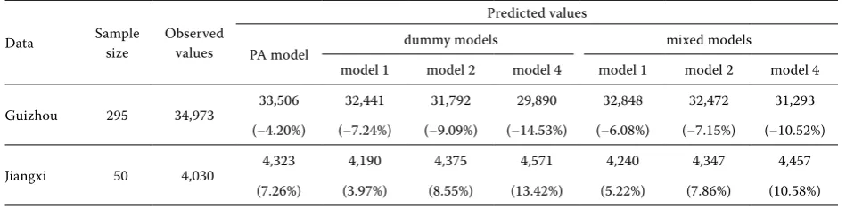
To examine the prediction results of the devel-oped models in this study, the authors used other aboveground biomass data from Masson pine plan-tations in Guizhou and Jiangxi provinces for

valida-tion. The prediction results of the models at differ-ent scales for validation data are listed in Table 6. It is shown in Table 6 that for validation data the predicted values of biomass in Guizhou are under-estimated for all models, and those in Jiangxi are overestimated; and the predicted results based on the PA model seem to be better. For the predicted values of dummy and mixed models, the smaller the scale, the larger the relative difference; and the bias of dummy model is larger than that of mixed model. In brief, the mixed model performed better than the dummy model for validation data.

From the properties of the models we know that mixed model is an intermediate form between the PA model and dummy model. In the PA model, the difference between various types such as origin and region was not taken into consideration; in dummy model, the difference between the types of sample was reflected by the fixed special parameters; and in mixed model, the difference was reflected by the random parameters based on the assumption that the data was distributed normally, and the random parameters could cancel out each other with an ex-pected value of zero. In fact, we can think that in mixed model the difference among various types of sample is divided into two parts: one originating from the difference among types; another resulting from the random effects. For example, the differ-ence between the two origins for the sample used in this study was 6.55% estimated by the dummy model, but in the mixed model, the difference was divided into two parts: 3.64% originating from the difference between natural and planted types, and the other 2.91% regarded as the random effects. We can expect that the fewer the sample trees in each type, the more numerous the random effects will be, and the mixed model will be closer to the PA model; and vice versa, the more numerous the sam-ple trees in each type, the fewer the random effects will be, and the mixed model will be closer to the dummy model.

Table 6. The prediction results of the models at different scales for validation data

Data Sample _size Observed _values

Predicted values

PA model dummy models mixed models

model 1 model 2 model 4 model 1 model 2 model 4

Guizhou 295 34,973 33,506 32,441 31,792 29,890 32,848 32,472 31,293

(–4.20%) (–7.24%) (–9.09%) (–14.53%) (–6.08%) (–7.15%) (–10.52%)

Jiangxi 50 4,030 4,323 4,190 4,375 4,571 4,240 4,347 4,457

(7.26%) (3.97%) (8.55%) (13.42%) (5.22%) (7.86%) (10.58%)

Possible limitation of the models

The emphasis of this study is mainly on meth-odology. The applicability of the developed mod-els was influenced by the sample size and repre-sentation. As for the size of the sample, a total of 150 trees from 9 provinces are adequate for devel-oping a generalized national or regional single-tree biomass model, but for sub-regional or provincial models the number of sample trees in each prov-ince is not sufficient. The reason is that 1–2 trees for each diameter class in each province are hardly the average on a provincial level. As for the rep-resentation of the sample, even though it was re-quired to select the sample trees by diameter class and by origin in each province, it was very difficult to assure the sample representative enough in prac-tice because of the small sample size and other fac-tors, which is reflected to some extent in Fig. 2. The modelling results show that single-tree biomass in natural forest is higher than that in plantation, which is probably because of better utilization of light, heat and water in natural forest. Tree biomass in the three south-eastern provinces (region 1) is higher than that in the three central provinces (re-gion 2), and the tree biomass in the three western and northern provinces (region 3) is the smallest. It is probably so because the water and heat con-ditions in the south-eastern region are better and the trees have enough growing space; but with the extension of the geographical region to west and north, the water and heat conditions are worse, which impacts the growth and development of the trees. If the combination of origins and regions is taken into consideration, the afore-mentioned gen-eral pattern is maintained no longer. For the natu-ral type, the tree biomass in region 2 is the smallest, and for the planted type, the biomass in region 2 is the largest, and the biomass of plantation in re-gion 2 is larger than that of natural forest. The rea-son is probably the small size and poor representa-tion of the sample for each type. Even though the models considering the combination of origins and regions and the PA model are different statistically, the special or random parameters are hardly differ-ent from zero (Tables 3 and 4), which show that the general pattern of tree biomass changing with the origins and regions is uncertain and up for valida-tion from a larger sample.

The dummy and mixed models used in this study are of logarithmic linear form which could be ex-tended to nonlinear models. Because the solution of nonlinear model is the asymptotic estimates based on Taylor’s series, the sum of predicted values

for fit data is not equal to that of observed values. In addition, the estimation of nonlinear biomass model involves the heteroscedasticity, i.e. the error term is multiplicative. All of these issues should be paid more attention, and for detailed discussion, see some related references (e.g. Laird et al. 1987; Pinherio, Bates 2000; Meng, Huang 2009).

COnCLUSIOnS

Based on the aboveground biomass data on Masson pine in Southern China, the generalized single-tree biomass equations suitable for national and regional forest biomass estimation were de-veloped using dummy model and linear mixed model methods, which could solve the compat-ibility of forest biomass estimates among differ-ent scales. The fitting results of subject-specific models showed that the aboveground biomass estimates of trees with the same diameter varied to some extent for different origins and for dif-ferent regions. For the Masson pine in Southern China, the aboveground biomass of a tree with the same diameter in natural forest was larger than that in plantation; and the biomass estimate de-creased from eastern region (Jiangsu, Zhejiang, Fujian) to south-central region (Jiangxi, Hunan, Guangdong) and to north-western region (Anhui, Guangxi, Guizhou). If considering the origins and regions together, different patterns would appear: for natural forests, trees with the same diameter in eastern regions have the largest biomass; and for plantations, trees in south-central regions have the largest biomass. But, because of the limited sample size, the conclusion above is subjected to valida-tion from a larger sample.

Acknowledgements

The authors express their appreciation to National Natural Science Foundation (No. 31070485 and No. 31170588) for financial support for this study. We also acknowledge the Central South Forest Inven-tory and Planning Institute of State Forestry Admin-istration of China for biomass data collection.

REFEREnCES

Baskerville G.L. (1972): Use of logarithmic regression in the estimation of plant biomass. Canadian Journal of Forest Research, 2: 49–53.

Case B., Hall R.J. (2008): Assessing prediction errors of generalized tree biomass and volume equations for the boreal forest region of west-central Canada. Canadian Journal of Forest Research, 38: 878–889.

Chojnacky D.C. (2002): Allometric scaling theory applied to FIA biomass estimation. In: McRoberts R.E., Reams G.A., Van Deusen P.C., Moser J.W. (eds): Proceedings of 3rd _{Annual Forest Inventory and Analysis Symposium.}

Traverse City, 17.–19. October 2001. St. Paul, North Central Research Station, Forest Service USDA, General Technical Report NC-230: 96–102.

FAO (2006): Global Forest Resources Assessment 2005: Progress Towards Sustainable Forest Management. FAO Forestry Paper 147. Rome, Food and Agriculture Organiza-tion of the United NaOrganiza-tions.

Fehrmann L., Lehtonen A., Kleinn C., Tomppo R. (2008): Comparison of linear and mixed-effect regression models and a k-nearest neighbor approach for estimation of single-tree biomass. Canadian Journal of Forest Research, 38: 1–9. Flewelling J.W., Pienaar L.V. (1981): Multiplicative regres-sion with lognormal errors. Forest Science, 27: 281–289. Fu L.Y., Zeng W.S., Tang S.Z. (2011): Analysis the effect of

region impacting on the biomass of domestic Masson pine using mixed model. Acta Ecologica Sinica, 31: 5797–5808. (in Chinese)

Gregoire T.G., Schabenberger O., Barrett J.P. (1995): Linear modeling of irregularly spaced, unbalanced, longitu-dinal data from permanent-plot measurements. Canadian Journal of Forest Research, 25: 137–156.

Hansen M. (2002): Volume and biomass estimation in FIA: National consistency vs. regional accuracy. In: McRoberts R.E., Reams G.A., Van Deusen P.C., Moser J.W. (eds): Proceedings of 3rd _{Annual Forest Inventory and Analysis}

Symposium. Traverse City, 17.–19. October 2001. St. Paul, North Central Research Station, Forest Service USDA, General Technical Report NC-230: 109–120.

Jenkins J.C., Chojnacky D.C., Heath L.S., Birdsey R.A. (2003): National-scale biomass estimators for United States tree species. Forest Science, 49: 12–35.

Laird N., Lange N., Stram D. (1987): Maximum likeli-hood computations with repeated measures: Application of the EM algorithm. Journal of the American Statistical Association, 82: 97–105.

Lang P.M. (2008): Linear mixed model of aerial photo crown width and ground diameter. Scientia Silvae Sinicae, 44: 41–44. (in Chinese)

Lappi J., Bailey R.L. (1988): A height prediction model with random stand and tree parameters: an alternative to tra-ditional site index methods. Forest Science, 38: 409–429. Lei X.D., Li Y.C., Xiang W. (2009): Individual basal area

growth model using multi-level linear mixed model with repeated measurements. Scientia Silvae Sinicae, 45: 74–80. (in Chinese)

Li X.H., Hong L.X. (1997): Research on the use of dummy variables method to calculate the family of site index curves. Forest Research, 10: 215–219. (in Chinese) Li C.M., Zhang H.R. (2010): Modeling dominant height for

Chinese fir plantation using a nonlinear mixed-effects mode-ling approach. Scientia Silvae Sinicae, 46: 89–95. (in Chinese) Li L.X., Hao Y.H., Zhang Y. (2006): The application of

dummy variable in statistic analysis. The Journal of Math-ematical Medicine, 19: 51–52. (in Chinese)

Li H., Mai J.Z., Xiao M. (2008): Application of dummy vari-able in logistic regression models. The Journal of Evidence-Based Medicine, 8: 42–45. (in Chinese)

Meng S.X., Huang S. (2009): Improved calibration of nonlin-ear mixed-effects models demonstrated on a height growth function. Forest Science, 55: 239–248.

Meng S.X., Huang S., Lieffers V.J. (2008): Wind speed and crown class influence the height-diameter relationship of lodgepole pine: Nonlinear mixed effects modeling. Forest Ecology and Management, 256: 570–577.

Muukkonen P. (2007): Generalized allometric volume and biomass equations for some tree species in Europe. Euro-pean Journal of Forest Research, 126: 157–166.

Návar J. (2009): Allometric equations for tree species and carbon stocks for forests of northwestern Mexico. Forest Ecology and Management, 257: 427–434.

Pinherio J.C., Bates D.M. (2000): Mixed-Effects Models in S and S-PLUS. New York, Springer-Verlag: 528.

Repola J., Ojansuu R., Kukkola M. (2007): Biomass func-tions for Scots pine, Norway spruce and birch in Finland. Working Papers of the Finnish Forest Research Institute, 53: 28. Available at http://www.metla.fi/julkaisut/working papers/2007/mwp053.htm

SAS Institute Inc. (1999): SAS/STAT User’s Guide, Ver- sion 8. Cary, SAS Institute Inc.

Snorrason A., Einarsson S.F. (2006): Single-tree biomass and stem volume functions for eleven tree species used in Icelandic forestry. Icelandic Agriculture Science, 19: 15–24. Snowdon P. (1991): A ratio estimator for bias correction

Tang S.Z., Li Y. (2002): Statistical Foundation for Biomath-ematical Models. Beijing, Science Press: 168–194. (in Chinese)

Tang S.Z., Lang K.J., Li H.K. (2008): Statistics and Computa-tion of Biomathematical Models (ForStat Course). Beijing, Science Press: 115–261. (in Chinese)

Ter-Mikaelian M.T., Korzukhin M.D. (1997): Biomass equations for sixty-five North American tree species. Forest Ecology and Management, 97: 1–24.

Tomppo E., Gschwantner T., Lawrence M., McRob-erts R.E. (2010): National Forest Inventories: Pathways for Common Reporting. 1st _{Ed. New York, Springer: 610.}

Vallet P., Dhôte J-F., Le Moguédec G., Ravart M., Pignard G. (2006): Development of total aboveground volume equations for seven important forest tree species in France. Forest Ecology and Management, 229: 98–110.

Wang M., Borders B.E., Zhao D. (2008): An empirical comparison of two subject-specific approaches to domi-nant heights modeling the dummy variable method and the mixed model method. Forest Ecology and Management, 255: 2659–2669.

West G.B., Brown J.H., Enquist B.J. (1999): A general model for the structure and allometry of plant vascular systems. Nature, 400: 664–667.

Zhang Y.J., Borders B.E. (2004): Using a system mixed-effects modeling method to estimate tree compartment biomass for intensively managed loblolly pines- an allo-metric approach. Forest Ecology and Management, 194: 145–157.

Received for publication September 14, 2011 Accepted after corrections December 13, 2011

Corresponding author:

Prof. Dr. Wei Sheng Zeng, Academy of Forest Inventory and Planning, State Forestry Administration, Hepingli Dongjie 18, Eastern District, Beijing, 100714, China