Learning local and global contexts using a convolutional recurrent network model for relation classification in biomedical text

Learning local and global contexts using a convolutional recurrent

network model for relation classification in biomedical text

Desh Raj and Sunil Kumar Sahu and Ashish Anand Department of Computer Science and Engineering

Indian Institute of Technology Guwahati Guwahati, India

Abstract

The task of relation classification in the biomedical domain is complex due to the presence of samples obtained from het-erogeneous sources such as research ar-ticles, discharge summaries, or electronic health records. It is also a constraint for classifiers which employ manual fea-ture engineering. In this paper, we pro-pose a convolutional recurrent neural net-work (CRNN) architecture that combines RNNs and CNNs in sequence to solve this problem. The rationale behind our ap-proach is that CNNs can effectively iden-tify coarse-grained local features in a sen-tence, while RNNs are more suited for long-term dependencies. We compare our CRNN model with several baselines on two biomedical datasets, namely the i2b2-2010 clinical relation extraction challenge dataset, and the SemEval-2013 DDI ex-traction dataset. We also evaluate an at-tentive pooling technique and report its performance in comparison with the con-ventional max pooling method. Our re-sults indicate that the proposed model achieves state-of-the-art performance on both datasets.1

1 Introduction

Relation classification is the task of identifying the semantic relation present between a given pair of entities in a piece of text. Since most search queries are some forms of binary fac-toids (Agichtein et al., 2005), modern question-answering systems rely heavily upon relation clas-sification as a preprocessing step (Fleischman

1_{The code for the can be found at:}

https://github.com/desh2608/ crnn-relation-classification.

et al., 2003;Lee et al., 2007). Accurate relation classification also facilitates discourse processing and precise sentence interpretations. Hence, this task has witnessed a great deal of attention over the last decade (Mintz et al.,2009;Surdeanu et al.,

2012).

In the biomedical domain, in particular, extract-ing such tuples from data may be essential for identifying protein and drug interactions, symp-toms and causes of diseases, among others. Fur-ther, since clinical data tends to be obtained from multiple (and diverse) information sources such as journal articles, discharge summaries, and elec-tronic patient records, relation classification be-comes a more challenging task.

To identify relations between entities, a vari-ety of lexical, syntactic, or pragmatic cues may be exploited, which results in a challenging vari-ability in the type of features used for classifi-cation purpose. Due to this variability, a num-ber of approaches have been suggested, some of which rely on features extracted from POS tag-ging, morphological analysis, dependency pars-ing, and world knowledge (Kambhatla,2004; San-tos et al., 2015; Suchanek et al., 2006; Mooney and Bunescu,2005;Bunescu and Mooney,2005). Deep learning architectures have recently gathered much interest because of their ability to conve-niently extract relevant features without the need of explicit feature engineering. For this reason, a number of convolutional and recurrent neural net-work models (Zeng et al.,2014;Xu et al.,2015b) have been used for this task.

In this paper, we propose a model that uses recurrent neural networks (RNNs) and convolu-tional neural networks (CNNs) in sequence to learn global and local context, respectively. We re-fer to this as CRNN, following the naming conven-tion used in (Huynh et al.,2016). We argue that in order for any classification task to be effective, the

regression layer must see a complete representa-tion of the sentence, i.e., both short and long-term dependencies must be appropriately represented in the sentence embedding. This argument forms the basis of our approach. In a deep learning frame-work, since the complete information available to the classifier at the top-level is obtained through manipulation of the sentence embedding itself, the task of relation classification essentially emulates other popular objectives such as text classification and sentiment analysis if the representation for the entity types are integrated in the sentence. Al-though our proposed model uses RNNs and CNNs in sequence, it is only two layers deep, as op-posed to the very deep architectures proop-posed ear-lier (Conneau et al., 2016). This simplicity al-lows for intuitive understanding of each level of the model, while still learning a sufficiently com-plex representation of the input sentence.

In addition to local and global contexts, we also experiment with attention for relation classifica-tion. Although attention as a concept is relatively well-known, especially in computational neuro-science (Itti et al., 1998; Desimone and Duncan,

1995), it became popular only recently with appli-cations to image captioning and machine transla-tion (Xu et al., 2015a;Vinyals et al., 2015; Bah-danau et al.,2014). Attention has also been em-ployed to some success in relation classification tasks (Wang et al.,2016a;Zhou et al.,2016a). In our experiments, we use an attention-based pool-ing strategy and compare the results with those ob-tained using conventional pooling methods. Our model variants are accordingly named CRNN-MaxandCRNN-Att, depending upong the pool-ing scheme used.

Our model is distinctive in that it does not rely upon any linguistic feature for relation clas-sification. In domains such as biomedicine, texts may not always be written in syntacti-cally/grammatically correct form. Furthermore, lack of necessary training data may not provide good feature extractors such as those in generic domains. Hence, we explored only models with-out any extra features. Of course, adding other fea-tures such as part-of-speech taggers or dependency parsers, if they are available easily, may improve the performance further. Our key contributions in this paper are as follows:

• We propose and validate a two-layer archi-tecture comprising RNNs and CNNs in

se-quence for relation classification in biomed-ical text. Our model’s performance is com-parable to the state-of-the-art on two bench-mark datasets, namely the i2b2-2010 clin-ical relation extraction challenge, and the SemEval-2013 DDI extraction dataset, with-out any need for handcrafted features.

• We analyze and discuss why such a model ef-fectively captures short and long-term depen-dencies in a sentence, and demonstrate why this representation facilitates classification.

• We evaluate an attention-based pooling tech-nique and compare its performance with con-ventional pooling strategies.

• We provide evidence to further the argument in favor of using RNNs to obtain regional em-beddings in a sentence.

2 Related Research

CNNs have been effectively employed in NLP tasks such as text classification (Kim,2014), sen-timent analysis (Dos Santos and Gatti,2014), re-lation classification (Zeng et al., 2014; Nguyen

and Grishman, 2015b), and so on. Similarly,

RNN models have also been used for similar tasks (Johnson and Zhang, 2016). The improved performance of these models is due to several rea-sons:

1. Pretrained word vectors are used as inputs for most of these models. These embed-dings capture the semantic similarity between words in a global context better than one-hot representations.

2. CNNs are capable of learning local features such as short phrases or recurring n-grams, similar to the way they provide translational, rotational and scale invariance in vision. 3. RNNs utilize the word order in the sentence,

and are also able to learn the long-term de-pendencies.

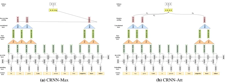
(a)CRNN-Max (b)CRNN-Att

Figure 1:Architecture of the proposed models. For representation purpose, the following configuration has been used:d=nO = 3,f1=f2= 2,nc= 4, and|C|= 3.

are then fed into an RNN layer which uses se-quence information to generate the sentence repre-sentation (Huynh et al.,2016;Wang et al.,2016b;

Chen et al.,2017;Nguyen and Grishman,2015a). These models are similar to ones that have also been employed to some success for visual recog-nition (Donahue et al.,2015). However, such mod-els are still limited because the RNN may “forget” features that occurred in the past if the sequence is very long.

We solve this problem by obtaining the output of the RNN at each time step (or word), and then pooling small phrases. This method of using a “re-current+pooling” module for regional embedding is inspired from (Johnson and Zhang,2016), who showed that for text categorization, embeddings of text regions, which can convey higher-level con-cepts than single words in isolation, are more use-ful than word embeddings. We also experiment with attention-pooling to integrate weighted fea-tures from discontinuous regions in the sentence.

3 Proposed Method

Given a sentenceSwith marked entitiese1ande2, belonging to entity types t1 andt2, respectively, and a set of relation classesC ={c1, . . . , cm}we

formulate the task of identifying the semantic re-lation as a supervised classification problem, i.e., we learn a function f : (S, E, T) → C, where S is the set of all sentences, E is the set of en-tity pairs, and T denotes the set of entity types. Our training objective is to learn a joint represen-tation of the sentence and the entity types, such that a softmax regression layer predicts the cor-rect label. To learn such an embedding, we pro-pose a two-layer neural network architecture

con-sisting of a “recurrent+pooling” layer and a “con-volutional+pooling” layer in sequence. This ar-chitecture is diagrammatically described in Fig.1, and the remainder of this section explains each of the layers in detail.

3.1 Embedding layer

The only features we use from S are the words themselves. The vector representation of these words is obtained using the GloVe method ( Pen-nington et al.,2014).

Pre-trained word vectors are used for the word embeddings and the words not present in the em-beddings list are initialized randomly. All the word vectors are updated during training.

3.2 Recurrent layer

RNN is a class of artificial neural networks which utilizes sequential information and maintains his-tory through its intermediate layers (Graves et al.,

2009). We use long short-term memory (LSTM) based model (Hochreiter and Schmidhuber,1997), which uses memory and gated mechanism to com-pute the hidden state. In particular we use a bidi-rectional LSTM model (Bi-LSTM) similar to the ones used in (Graves,2013;Huang et al.,2015).

Let h(_lt) andh(rt) be the outputs obtained from

the forward and backward direction of the LSTM at timet. Then the combined output is given as

z(t)=h(_lt):h_r(t), z(t) ∈RnO_{. (1)}

3.3 First pooling layer

The recurrent layer generates word-level embed-dings that incorporate information from the past and future context. Sometimes the word itself may not be important for the sentence representation, and in such cases, it may be better to extract the most important features from short phrases using a pooling technique. If f1 denotes the length of the filter used for pooling, and(z1, . . . , zm)is the

sequence of vectors obtained from the previous layer, then

p= (p1, p2, . . . , pm−f1+1), (2)

wherepi ∈RnO is given as pi = max

1≤j≤f1[zi+j], (3)

i.e. the maximum among all vectorszi+1tozi+f1.

3.4 Convolutional layer

We apply convolution on p to get local features from each part of the sentence (Collobert and

Weston, 2008). Consider a convolutional filter

parametrized by weight vector wc ∈ RnO∗f2,

where f2 is the length of filter. Then the output sequence of convolution layer would be

hi_c=f(wc·pi:i+f2−1+bc), (4)

where i = 1,2, . . . , m−f1 −f2 + 2, · is dot product,f is the rectifier linear unit (ReLU) func-tion (f(x) = max{0, x}), andbc ∈ Ris the bias

term. The parameterswcandbcare shared across

all convolutions i = 1,2, . . . , m−f1−f2 + 2. On applying nc such filters, we obtain an output

matrixHc∈Rnc×(m−f1−f2+2). 3.5 Second pooling layer

The output of the convolutional layer is of vari-able length (m−f1 −f2 + 2), since it depends on the length m of the input sentence. To ob-tain fixed length global features for the entire sen-tence, we apply pooling over the entire sequence. For this, we experiment with two different pool-ing schemes based on which our model has two variations, namely CRNN-Max and CRNN-Att. 3.5.1 Max pooling over time

Max pooling over time (Collobert and Weston,

2008) takes the maximum over the entire sentence, with the assumption that all the relevant informa-tion is accumulated in that posiinforma-tion. Since the in-put to this layer are the local convolved vectors,

this strategy essentially extracts the most impor-tant features from several short phrases. The out-put is then given as

zpool = max

1≤i≤(m−f1−f2+2)[h

i

c], (5)

where zpool ∈ Rnc is the dimension-wise

maxi-mum over allhi c’s.

3.5.2 Attention-based pooling

A max pooling scheme may fail when impor-tant cues are distributed across different clauses in the sentence. We solve this problem by us-ing an attention-based poolus-ing scheme, which ob-tains an optimal feature dimension-wise by tak-ing weighted linear combinations of the vec-tors. These weights are trained using an atten-tion mechanism such that more important fea-tures are weighed higher (Bahdanau et al., 2014;

Yang et al., 2016; Zhou et al., 2016b). The at-tention mechanism produces a vector α of size m −f1 −f2 + 2, and the values in this vector are the weights for each phrase obtained from the convolutional layer feature vectors.

Hatt= tanh(W1αHc) α=Softmax(W₂αTHatt)

zatt=αHcT (6)

Here, Hc is the matrix of CNN output

vec-tors,Wα

1, W2α ∈Rnc×nc is the parameter matrix,

α ∈ Rm−f1−f2+2 are the attention weights, and

zatt ∈Rnc is the output of the pooling layer. The

attention weights are a function of the input sen-tence, and henceαis different for every sentence. 3.6 Fully connected and softmax

To obtain a classifier over the extracted global fea-tures, we use a fully connected layer consisting of

|C|nodes, whereCis the set of all possible rela-tion classes, followed by a softmax layer to gen-erate a probability distribution over the set of all possible labels. The final output is given as

p(ci|x) =Softmax(Wioz+boi), (7)

whereWo_andbo _{are the weight and bias}

param-eters, and z may be either zpool or zatt,

depend-ing on the second pooldepend-ing layer scheme. The pre-dicted outputy0_{is obtained as}

y0= arg max

ci∈C

Class Train size Test size

TrCP 436 108 TrAP 2131 532

TrWP 109 26

TrIP 165 41 TrNAP 140 34 TeRP 2457 614 TeCP 409 101 PIP 1776 443 None 44588 11146

Total 52211 13045

Table 1: Number of training and testing instances for each relation type in the i2b2 dataset.

4 Experiments

4.1 Datasets

We have used 2 datasets for experimentation, namely the i2b2-2010 clinical relation extrac-tion challenge dataset (Sun et al., 2013), and the SemEval-2013 DDI extraction dataset ( Se-gura Bedmar et al.,2013).

i2b2-2010 relation extraction

This dataset contains sentences from discharge summaries collected from three different hospi-tals and have 8 relation types: treatment caused medical problems(TrCP),treatment administered medical problem(TrAP),treatment worsen med-ical problem(TrWP),treatment improve or cure medical problem (TrIP), treatment was not ad-ministered because of medical problem(TrNAP),

test reveal medical problem (TeRP), test con-ducted to investigate medical problem (TeCP), and medical problem indicates medical problem

(PIP). If a sentence has more than two entities, we make an instance for each pair. Since only 170 of the 394 original training documents and 256 of the 477 testing documents were available for down-load, we combined all the training and testing in-stances, and then split it in a 80:20 ratio for train-ing and test sets respectively. The statistics of the dataset are described in Table1.

SemEval 2013 DDI extraction

This dataset contains annotated sentences from two sources, Medline abstracts (biomedical re-search articles) and DrugBank database (docu-ments written by medical practitioners). The dataset is annotated with following four kinds of interactions: advice (opinion or consultation re-lated to the simultaneous use of the two drugs),

effect (effect of the DDI together with pharma-codynamic effect or mechanism of interaction),

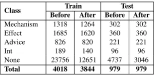
Class _{Before After Before After}Train Test Mechanism 1318 1264 302 302 Effect 1685 1620 360 360 Advice 826 820 221 221 Int 189 140 96 96 None 23756 12651 4737 3046 Total 4018 3844 979 979

Table 2: Number of training and testing instances for each relation type in the DDI extraction dataset.

mechanism(pharmacokinetic mechanism), andint

(drug interaction without any other information). Dataset provides the training and test instances by sentences. Similar to i2b2 relation extrac-tion dataset if a sentence has more than two drug names, all possible pairs of drugs in the sentence have been separately annotated, such that a single sentence having multiple drug names leads to sep-arate instances of drug pairs and corresponding in-teraction. Statistics of the dataset (along with neg-ative instance filtering, discussed in Section4.1.1) is shown in Table2.

4.1.1 Preprocessing

As a preprocessing step, we replace the enti-ties in the i2b2 dataset with the corresponding entity types. For instance, the sentence: “He was given Lasix to prevent him from conges-tive heart failure.” was converted to: “He was givenTREATMENT Ato prevent him from PROB-LEM B.” Similarly, for the DDI extraction dataset, the two targeted drug names are replaced with DRUG-A and DRUG-B respectively, and other drug names in the same sentence are replaced with DRUG-N. Further, all numbers were replaced with the keyword NUM. Similar to the earlier studies (Sahu and Anand, 2017;Liu et al.,2016;

Rastegar-Mojarad et al.,2013), negative instances were filtered from training sets.

4.2 Implementation details

val-ues of 0.01 (0.001) and 0.7 (0.5) were found op-timal for the regularization parameter and dropout for the i2b2 (DDI extraction) dataset, respectively. We use Adam technique (Kingma and Ba,2014) to optimize our loss function, with a learning rate of 0.01. For all the models,nOandnC were tuned

on the validation set, and values of 200 and 100 were found to be optimal. Hyperparameters of baseline methods were taken from the values sug-gested in the respective papers. Entire neural net-work parameters and feature vectors are updated while training. We have implemented the pro-posed model in Python language using the Tensor-flow package (Abadi et al.,2016). We experiment with different filter sizes forf1andf2 and discuss the results in Section5.1.

4.3 Baseline methods

We compare our models with 5 methods that have earlier been used for relation classification to satis-factory results. These baselines were selected for one of the following three purposes.

Feature-based methods

We selected a feature-based SVM classifier (Rink et al.,2011) that uses several handcrafted features such as distance of word from entities, POS tags, chunk tags, etc., to compare whether our mod-els were able to outperform classifiers with rigor-ous feature engineering. It is to be noted that we use our own implementation of the SVM classifier (using the scikit-learn (Pedregosa et al., 2011) li-brary), using features as described in (Sahu et al.,

2016).

Single-layer neural networks

We selected a multiple-filter CNN with max-pooling (Sahu et al., 2016) and an LSTM model with max and attentive pooling (Sahu and Anand,

2017). In Section 5.5, we compare our models with these single layer models to justify using a combination of RNN and CNN to learn long-term and short-term dependencies, respectively. To ob-serve the effect of the network model independent of the feature set, we use only the word embed-dings as features for each of these models. Further, we used the same hyperparameters as mentioned in the respective papers.

Recurrent convolutional neural network This model, inspired from (Wang et al., 2016b), obtains regional embeddings using a convolutional

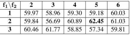
f1\f2 2 3 4 5 6

1 59.97 58.96 59.30 59.18 60.03

2 59.84 56.69 60.89 62.45 61.03

3 60.46 61.77 58.85 57.34 59.81

Table 3:Average F1 scores on varying filter sizesf1andf2

in the CRNN-Att model for i2b2 dataset.

layer. These are then fed into a recurrent layer and a single output is obtained after traversing the en-tire sequence. We compare our models with this RCNN model to observe the effect of obtaining outputs at every word, as opposed to at the end of the sequence.

5 Results and Discussion

5.1 Effect of filter sizesf1andf2

We experiment with various combinations of fil-ter sizesf1 andf2 on the i2b2 dataset using our CRNN-Att model. Since f1 denotes the size of the first pooling filter, it essentially represents the amount of information present in a regional em-bedding that is fed into the convolutional layer. If f1 is too small (f1 = 1, i.e., no pooling), em-beddings from seemingly unimportant words may get through, and if it is large (f1 ≥ 3), individ-ual embeddings may get pooled such that a few words dominate the majority of regions. For the filter size f2 in the convolutional layer, a mid-range value (4 to 6) was found to work well. This may be because this layer learns to identify short phrases which are usually of this length. These observations were common for both datasets. The F1 scores for various combinations of filter sizes on the i2b2 data are shown in Table3. In the re-maining experiments, we choose (f1,f2) = (2,5) for both our model variants.

5.2 Initialization and tuning of word embeddings

The only feature used in our models is the word vectors for every word in the sentence. We per-form several experiments on the i2b2 data to ob-serve the effect of word vector initialization and update on the model performance. The results are summarized in Table5.

Interestingly, the best performing model uses randomly initialized word embeddings that are not updated during training. This is in contrast to earlier studies (Sahu and Anand,2017;Collobert

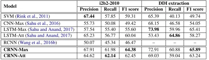
Model _{Precision Recall F1 score Precision Recall F1 score}i2b2-2010 DDI extraction

SVM (Rink et al.,2011) 67.44 57.85 59.31 65.39 40.13 49.74 CNN-Max (Sahu et al.,2016) 55.73 50.08 49.42 68.15 46.58 54.05 LSTM-Max (Sahu and Anand,2017) 57.54 55.40 55.60 73.98 59.96 65.41 LSTM-Att (Sahu and Anand,2017) 65.23 56.77 60.04 53.43 64.86 58.27 RCNN (Wang et al.,2016b) 50.07 45.34 46.47 – – –

CRNN-Max 67.91 61.98 64.38 72.91 60.88 65.89

CRNN-Att 64.62 62.14 62.45 69.03 59.04 63.24

Table 4:Comparison of our proposed models CRNN-Max and CRNN-Att, with baselines, on the i2b2-2010 and DDI extraction datasets.

Initialization update CRNN-Max CRNN-Att

Random Trainable 62.78 61.19 Random Non-trainable 64.38 61.51 PubMed Trainable 60.60 62.45

PubMed Non-trainable 58.49 59.35

Table 5: Effect of initialization and update of word embed-dings in our proposed models, in terms of F1 score, using the i2b2-2010 datset.

Class Size SVM CNN LSTM-Max RCNN CRNN-Max CRNN-Att

TrCP 108 34.90 34.01 35.48 18.30 43.18 47.66

TrAP 532 63.48 46.69 58.74 45.15 67.39 63.94 TrWP 26 7.41 10.26 0.00 0.00 16.67 9.52 TrIP 41 9.09 21.74 0.00 0.00 25.71 34.48

TrNAP 34 5.13 15.87 0.00 0.00 36.36 18.60 TeRP 614 80.44 63.52 73.50 67.01 80.32 76.31 TeCP 101 30.30 27.63 25.20 11.48 39.46 39.76

PIP 443 49.44 49.30 51.54 45.05 58.04 55.53

Table 6: Classwise performance (in terms of F1 score) of various models on the i2b2 dataset.

usually improved model performances by 3-4%. However, this result aligns with the observations made in (Johnson and Zhang,2015) and supports the argument for one-hot LSTMs. It may be en-lightening to discuss why such a result is obtained. First, we note that in the formulas for LSTM, e.g., ut = tanh(W(u)xt + U(u)ht−1 + b(u)), if xt is the one-hot representation of a word, the

termW(u)_{xt serves as a word embedding. Thus,} a one-hot LSTM inherently includes a word em-bedding in its computation. Further, a word vector lookup is a linear operation, and hence it may be merged into the LSTM layer itself by multiplying the LSTM weights by the word embedding matrix. This means that the expressive power of an LSTM which uses pretrained vectors is the same as that of one which uses randomly initialized word em-beddings. It has also been shown in earlier stud-ies that pretrained embeddings do not improve the performance of networks as the number of layers increases.

Johnson et al. (2015) even argued that the em-bedding layer can be replaced with a one-hot

representation without compromising on the per-formance. Empirically, inclusion of an embed-ding layer makes training from scratch more diffi-cult, even with the help of adaptive learning rates. Similar observations have been made regarding CNNs (Kim,2014;Johnson and Zhang,2014). 5.3 Comparison with baseline methods Table4shows the results obtained on the i2b2 and DDI extraction datasets using our proposed mod-els, as compared to the baseline methods. Our models outperform the baselines even without the need for explicit feature engineering. It is interest-ing to note that our CRNN-Max performs better than the CRNN-Att, and a similar result has also been observed earlier in (Sahu and Anand,2017). Class-wise performance analysis

We compare class-wise performance of our mod-els on the i2b2 dataset with some of the baselines, and this is summarized in Table 6. It is evident that performances improve with training size, and from the confusion matrices (not shown here), we found that samples of a lower frequency class were misclassified into a higher frequency class com-prising the same entity types. For instance, sam-ples belonging to TrWP (Treatment Worsen medi-cal Problem) were often classified as TrAP (Treat-ment Administered medical Problem).

5.4 Effect of attention-based pooling

Figure 2:Attention heatmap for 5 sentences selected from the i2b2-2010 dataset. A darker background corresponds to a larger attention weight.

of weights of all phrases that the word is present in. The figure shows that the attentive pooling scheme is able to select important phrases depend-ing upon the classification label. It is evident that the model assigns a higher weight to semantically relevant words such as “showed,” “question,” and “revealed”.

5.5 Long and short term dependencies

We conjecture that our proposed CRNN models perform better than single layer CNNs or RNNs because they capture both local and global con-texts efficiently. To confirm our hypothesis, we determine the average sentence lengths and entity separations for several sets of sentences belong-ing to classes where our models performed well, and for classes where either the CNN model or the LSTM-Max model performed relatively well, for the i2b2-2010 dataset. These results are visualized in the box plots shown in Fig.3.

From the figure, we note that our models CRNN-Max and CRNN-Att perform significantly better than a CNN model in classifying long sen-tences with large entity separation, while CNN models work well with shorter sentences where the entities are less separated. This is evident by observing the median and range of lower to up-per quartile values in the figure. This confirms our conjecture that our models learn long-term dependencies better than a simple CNN model. Similarly, our proposed models perform better on a larger range of sentence lengths than LSTMs, which may be due to more effective modeling of local contexts.

(a)

(b)

Figure 3: Box plots for distribution of (a) sentence lengths and (b) entity separation for sentence sets. A representation of the form{X}\{˜Y}denotes the set of sentences correctly classified by model X but wrongly classified by model Y. The numbers at the top are the median values for each box.

5.6 Effect of linguistic features

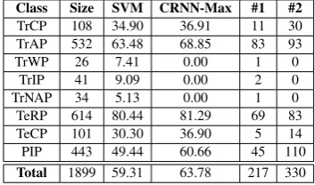
Class Size SVM CRNN-Max #1 #2 TrCP 108 34.90 36.91 11 30 TrAP 532 63.48 68.85 83 93

TrWP 26 7.41 0.00 1 0

TrIP 41 9.09 0.00 2 0

TrNAP 34 5.13 0.00 1 0

TeRP 614 80.44 81.29 69 83 TeCP 101 30.30 36.90 5 14 PIP 443 49.44 60.66 45 110 Total 1899 59.31 63.78 217 330

Table 7: Classwise performance comparison between SVM and CRNN-Max using linguistic features. #1 denotes num-ber of sentences of a class classified correctly by SVM but incorrectly by CRNN-Max; #2 denotes vice-versa.

by replacing the entities with their corresponding types. Furthermore, we have also described ex-periments with initialization and update of word embeddings.

In this section, we add the four other linguis-tic features in our proposed model to observe its performance in comparison with the SVM model. Table7summarizes this comparison.

Although the F1 scores for the models are rel-atively close, the precision (P) and recall (R) vary significantly: P is 67.44 and 61.00, while R is 57.85 and 67.54, for the SVM and CRNN-Max models, respectively. Our CRNN-Max model, therefore, is more sensitive while the SVM clas-sifier has a higher specificity. Furthermore, it is evident that SVM outperforms our model only on classes with a disproportionately low instance count. We may argue that due to the presence of more features and less number of records, our model gets over-trained only on the larger classes. This problem may then be avoided with better reg-ularization, to achieve even higher performance.

6 Conclusion

In this work, we proposed and evaluated a two-layer architecture comprising recurrent and con-volutional layers in sequence to learn global and local contexts in a sentence, which was then used for relation classification. To the best of our knowledge, this is the first attempt at com-bining CNNs and RNNs in sequence for a re-lation classification task in biomedical domain. Two variants of the model, namely CRNN-Max and CRNN-Att, were evaluated on the i2b2-2010 dataset and the SemEval 2013 DDI extraction dataset, and max-pooling was found to perform better than attentive pooling. Even though our method employed only word embeddings as

in-put feature, it was able to conveniently outper-form state-of-the-art techniques that use extensive feature engineering. Finally, our results indicated that a “recurrent+pooling” layer effectively gener-ates regional embedding without the need for pre-trained word vectors. It would be interesting to see whether one-hot word vectors perform better than randomly initialized embeddings. We may also benefit from probing whether tree-based or non-continuous convolutions work as well as our CRNN models for learning long and short term de-pendencies for relation classification.

References

Martın Abadi, Ashish Agarwal, Paul Barham, Eugene Brevdo, Zhifeng Chen, Craig Citro, Greg S Corrado, Andy Davis, Jeffrey Dean, Matthieu Devin, et al. 2016. Tensorflow: Large-scale machine learning on

heterogeneous distributed systems. arXiv preprint

arXiv:1603.04467.

Eugene Agichtein, Silviu Cucerzan, and Eric Brill. 2005. Analysis of factoid questions for effective relation extraction. InProceedings of the 28th an-nual international ACM SIGIR conference on Re-search and development in information retrieval. ACM, pages 567–568.

Dzmitry Bahdanau, Kyunghyun Cho, and Yoshua Ben-gio. 2014. Neural machine translation by jointly

learning to align and translate. arXiv preprint

arXiv:1409.0473.

Razvan C Bunescu and Raymond J Mooney. 2005. A shortest path dependency kernel for relation

extrac-tion. In Proceedings of the conference on human

language technology and empirical methods in nat-ural language processing. Association for Compu-tational Linguistics, pages 724–731.

Guibin Chen, Deheng Ye, Erik Cambria, Jieshan Chen, and Zhenchang Xing. 2017. Ensemble application of convolutional and recurrent neural networks for multi-label text categorization. IJCNN.

Ronan Collobert and Jason Weston. 2008. A unified architecture for natural language processing: Deep

neural networks with multitask learning. In

Pro-ceedings of the 25th international conference on Machine learning. ACM, pages 160–167.

Alexis Conneau, Holger Schwenk, Lo¨ıc Barrault, and Yann Lecun. 2016. Very deep convolutional

net-works for natural language processing. arXiv

preprint arXiv:1606.01781.

Jeffrey Donahue, Lisa Anne Hendricks, Sergio Guadar-rama, Marcus Rohrbach, Subhashini Venugopalan, Kate Saenko, and Trevor Darrell. 2015. Long-term recurrent convolutional networks for visual

recogni-tion and descriprecogni-tion. In Proceedings of the IEEE

conference on computer vision and pattern recogni-tion. pages 2625–2634.

C´ıcero Nogueira Dos Santos and Maira Gatti. 2014. Deep convolutional neural networks for sentiment analysis of short texts. InCOLING. pages 69–78. Michael Fleischman, Eduard Hovy, and Abdessamad

Echihabi. 2003. Offline strategies for online ques-tion answering: Answering quesques-tions before they

are asked. InProceedings of the 41st Annual

Meet-ing on Association for Computational LMeet-inguistics- Linguistics-Volume 1. Association for Computational Linguis-tics, pages 1–7.

Alex Graves. 2013. Generating sequences with

recurrent neural networks. arXiv preprint

arXiv:1308.0850.

Alex Graves, Marcus Liwicki, Santiago Fern´andez, Roman Bertolami, Horst Bunke, and J¨urgen Schmidhuber. 2009. A novel connectionist system

for unconstrained handwriting recognition. IEEE

transactions on pattern analysis and machine intel-ligence31(5):855–868.

Sepp Hochreiter and J¨urgen Schmidhuber. 1997.

Long short-term memory. Neural computation

9(8):1735–1780.

Zhiheng Huang, Wei Xu, and Kai Yu. 2015.

Bidirec-tional lstm-crf models for sequence tagging. arXiv

preprint arXiv:1508.01991.

Trung Huynh, Yulan He, Allistair Willis, and Stefan R¨uger. 2016. Adverse drug reaction classification with deep neural networks .

Laurent Itti, Christof Koch, Ernst Niebur, et al. 1998. A model of saliency-based visual attention for rapid

scene analysis. IEEE Transactions on pattern

anal-ysis and machine intelligence20(11):1254–1259.

Rie Johnson and Tong Zhang. 2014. Effective

use of word order for text categorization with

convolutional neural networks. arXiv preprint

arXiv:1412.1058.

Rie Johnson and Tong Zhang. 2015. Semi-supervised convolutional neural networks for text

categoriza-tion via region embedding. InAdvances in neural

information processing systems. pages 919–927.

Rie Johnson and Tong Zhang. 2016.

Super-vised and semi-superSuper-vised text categorization

us-ing lstm for region embeddus-ings. arXiv preprint

arXiv:1602.02373.

Nanda Kambhatla. 2004. Combining lexical, syntac-tic, and semantic features with maximum entropy

models for extracting relations. InProceedings of

the ACL 2004 on Interactive poster and demonstra-tion sessions. Association for Computational Lin-guistics, page 22.

Yoon Kim. 2014. Convolutional neural

net-works for sentence classification. arXiv preprint

arXiv:1408.5882.

Diederik Kingma and Jimmy Ba. 2014. Adam: A

method for stochastic optimization. arXiv preprint

arXiv:1412.6980.

Changki Lee, Yi-Gyu Hwang, and Myung-Gil Jang. 2007. Fine-grained named entity recognition and relation extraction for question answering. In Pro-ceedings of the 30th annual international ACM SI-GIR conference on Research and development in in-formation retrieval. ACM, pages 799–800.

Shengyu Liu, Buzhou Tang, Qingcai Chen, and Xiao-long Wang. 2016. Drug-drug interaction extraction

via convolutional neural networks. Computational

and mathematical methods in medicine2016.

Mike Mintz, Steven Bills, Rion Snow, and Dan Ju-rafsky. 2009. Distant supervision for relation

ex-traction without labeled data. In Proceedings of

the Joint Conference of the 47th Annual Meeting of the ACL and the 4th International Joint Conference on Natural Language Processing of the AFNLP: Volume 2-Volume 2. Association for Computational Linguistics, pages 1003–1011.

Raymond J Mooney and Razvan C Bunescu. 2005. Subsequence kernels for relation extraction. In Ad-vances in neural information processing systems. pages 171–178.

TH Muneeb, Sunil Kumar Sahu, and Ashish Anand. 2015. Evaluating distributed word representations for capturing semantics of biomedical concepts.

Proceedings of ACL-IJCNLPpage 158.

Thien Huu Nguyen and Ralph Grishman. 2015a. Combining neural networks and log-linear

mod-els to improve relation extraction. arXiv preprint

arXiv:1511.05926.

Thien Huu Nguyen and Ralph Grishman. 2015b. Rela-tion extracRela-tion: Perspective from convoluRela-tional

neu-ral networks. InProceedings of NAACL-HLT. pages

39–48.

F. Pedregosa, G. Varoquaux, A. Gramfort, V. Michel, B. Thirion, O. Grisel, M. Blondel, P. Pretten-hofer, R. Weiss, V. Dubourg, J. Vanderplas, A. Pas-sos, D. Cournapeau, M. Brucher, M. Perrot, and E. Duchesnay. 2011. Scikit-learn: Machine learning

in Python. Journal of Machine Learning Research

12:2825–2830.

Jeffrey Pennington, Richard Socher, and Christopher D Manning. 2014. Glove: Global vectors for word

representation. InEMNLP. volume 14, pages 1532–

Majid Rastegar-Mojarad, Richard D Boyce, and Rashmi Prasad. 2013. UWM-TRIADS: classify-ing drug-drug interactions with two-stage SVM and

post-processing. In Proceedings of the 7th

Inter-national Workshop on Semantic Evaluation. pages 667–674.

Bryan Rink, Sanda Harabagiu, and Kirk Roberts. 2011. Automatic extraction of relations between medical concepts in clinical texts. Journal of the American Medical Informatics Association18(5):594–600. Sunil Kumar Sahu and Ashish Anand. 2017.

Drug-drug interaction extraction from biomedical text

us-ing long short term memory network. arXiv preprint

arXiv:1701.08303.

Sunil Kumar Sahu, Ashish Anand, Krishnadev Oru-ganty, and Mahanandeeshwar Gattu. 2016. Relation extraction from clinical texts using domain

invari-ant convolutional neural network. arXiv preprint

arXiv:1606.09370.

Cicero Nogueira dos Santos, Bing Xiang, and Bowen Zhou. 2015. Classifying relations by ranking with

convolutional neural networks. arXiv preprint

arXiv:1504.06580.

Isabel Segura Bedmar, Paloma Mart´ınez, and Mar´ıa Herrero Zazo. 2013. Semeval-2013 task 9: Ex-traction of drug-drug interactions from biomedical texts (ddiextraction 2013). Association for Compu-tational Linguistics.

Nitish Srivastava, Geoffrey E Hinton, Alex Krizhevsky, Ilya Sutskever, and Ruslan Salakhutdinov. 2014. Dropout: a simple way to prevent neural networks

from overfitting. Journal of Machine Learning

Re-search15(1):1929–1958.

Fabian M Suchanek, Georgiana Ifrim, and Gerhard Weikum. 2006. Combining linguistic and statistical analysis to extract relations from web documents. In Proceedings of the 12th ACM SIGKDD interna-tional conference on Knowledge discovery and data mining. ACM, pages 712–717.

Weiyi Sun, Anna Rumshisky, and Ozlem Uzuner. 2013. Evaluating temporal relations in clinical text: 2012

i2b2 challenge. Journal of the American Medical

Informatics Association20(5):806–813.

Mihai Surdeanu, Julie Tibshirani, Ramesh Nallapati, and Christopher D Manning. 2012. Multi-instance multi-label learning for relation extraction. In Pro-ceedings of the 2012 Joint Conference on Empirical

Methods in Natural Language Processing and Com-putational Natural Language Learning. Association for Computational Linguistics, pages 455–465.

Oriol Vinyals, Alexander Toshev, Samy Bengio, and Dumitru Erhan. 2015. Show and tell: A neural

im-age caption generator. InProceedings of the IEEE

Conference on Computer Vision and Pattern Recog-nition. pages 3156–3164.

Linlin Wang, Zhu Cao, Gerard de Melo, and Zhiyuan Liu. 2016a. Relation classification via multi-level attention cnns. InACL.

Xingyou Wang, Weijie Jiang, and Zhiyong Luo. 2016b. Combination of convolutional and recurrent neural network for sentiment analysis of short texts. In

Proceedings of the 26th International Conference on Computational Linguistics. pages 2428–2437.

Kelvin Xu, Jimmy Ba, Ryan Kiros, Kyunghyun Cho, Aaron Courville, Ruslan Salakhutdinov, Richard S Zemel, and Yoshua Bengio. 2015a. Show, attend and tell: Neural image caption generation with

vi-sual attention. arXiv preprint arXiv:1502.03044

2(3):5.

Kun Xu, Yansong Feng, Songfang Huang, and Dongyan Zhao. 2015b. Semantic relation clas-sification via convolutional neural networks

with simple negative sampling. arXiv preprint

arXiv:1506.07650.

Zichao Yang, Diyi Yang, Chris Dyer, Xiaodong He, Alex Smola, and Eduard Hovy. 2016. Hierarchical attention networks for document classification. In

Proceedings of NAACL-HLT. pages 1480–1489.

Daojian Zeng, Kang Liu, Siwei Lai, Guangyou Zhou, Jun Zhao, et al. 2014. Relation classification via

convolutional deep neural network. In COLING.

pages 2335–2344.

Peng Zhou, Wei Shi, Jun Tian, Zhenyu Qi, Bingchen Li, Hongwei Hao, and Bo Xu. 2016a. Attention-based bidirectional long short-term memory net-works for relation classification. InACL.