Predefined Sparseness in Recurrent Sequence Models

Proceedings of the 22nd Conference on Computational Natural Language Learning (CoNLL 2018), pages 324–333 324

Predefined Sparseness in Recurrent Sequence Models

Thomas Demeester, Johannes Deleu, Fr´ederic Godin, Chris Develder Ghent University - imec

Ghent, Belgium

[email protected]

Abstract

Inducing sparseness while training neural net-works has been shown to yield models with a lower memory footprint but similar effective-ness to dense models. However, sparseeffective-ness is typically induced starting from a dense model, and thus this advantage does not hold during training. We propose techniques to enforce sparseness upfront in recurrent sequence mod-els for NLP applications, to also benefit train-ing. First, in language modeling, we show how to increase hidden state sizes in recurrent lay-ers without increasing the number of parame-ters, leading to more expressive models. Sec-ond, for sequence labeling, we show that word embeddings with predefined sparseness lead to similar performance as dense embeddings, at a fraction of the number of trainable parameters.

1 Introduction

Many supervised learning problems today are solved with deep neural networks exploiting large-scale labeled data. The computational and mem-ory demands associated with the large amount of parameters of deep models can be alleviated by us-ing sparse models. Applying sparseness can be seen as a form of regularization, as it leads to a reduced amount of model parameters1, for given layer widths or representation sizes. Current suc-cessful approaches gradually induce sparseness during training, starting from densely initialized networks, as detailed in Section 2. However, we propose that models can also be built with pre-defined sparseness, i.e., such models are already sparse by design and do not require sparseness in-ducing training schemes.

The main benefit of such an approach is mem-ory efficiency, even at the start of training. Espe-cially in the area of natural language processing, in

1_{The sparseness focused on in this work, occurs on the} level of trainable parameters, i.e., we do not consider data sparsity.

line with the hypothesis byYang et al.(2017) that natural language is “high-rank”, it may be useful to train larger sparse representations, even when facing memory restrictions. For example, in order to train word representations for a large vocabu-lary using limited computational resources, prede-fined sparseness would allow training larger em-beddings more effectively compared to strategies inducing sparseness from dense models.

The contributions of this paper are (i) a predefined sparseness model for recurrent neu-ral networks, (ii) as well as for word embed-dings, and (iii) proof-of-concept experiments on part-of-speech tagging and language modeling, in-cluding an analysis of the memorization capacity of dense vs. sparse networks. An overview of re-lated work is given in the next Section2. We sub-sequently present predefined sparseness in recur-rent layers (Section3), as well as embedding lay-ers (Section 4), each illustrated by experimental results. This is followed by an empirical investi-gation of the memorization capacity of language models with predefined sparseness (Section 5). Section 6 summarizes the results, and points out potential areas of follow-up research.

The code for running the presented experiments is publically available.2

2 Related Work

A substantial body of work has explored the bene-fits of using sparse neural networks. In deep con-volutional networks, common approaches include sparseness regularization, e.g., using decompo-sition (Liu et al., 2015) or variational dropout (Molchanov et al.,2017)), pruning of connections (Han et al.,2016,2015;Guo et al.,2016) and low rank approximations (Jaderberg et al., 2014; Tai et al., 2016). Regularization and pruning often

lead to mostly random connectivity, and therefore to irregular memory accesses, with little practical effect in terms of hardware speedup. Low rank approximations are structured and thus do achieve speedups, with as notable examples the works of

Wen et al. (2016) and Lebedev and Lempitsky

(2016).

Whereas above-cited papers specifically ex-plored convolutional networks, our work focuses on recurrent neural networks (RNNs). Similar ideas have been applied there, e.g., see Lu et al.

(2016) for a systematic study of various new com-pact architectures for RNNs, including low-rank models, parameter sharing mechanisms and struc-tured matrices. Also pruning approaches have been shown to be effective for RNNs, e.g., by

Narang et al.(2017). Notably, in the area of audio synthesis,Kalchbrenner et al.(2018) showed that large sparse networks perform better than small dense networks. Their sparse models were ob-tained by pruning, and importantly, a significant speedup was achieved through an efficient imple-mentation.

For the domain of natural language processing (NLP), recent work by Wang et al. (2016) pro-vides an overview of sparse learning approaches, and in particular noted that “application of sparse coding in language processing is far from exten-sive, when compared to speech processing”. Our current work attempts to further fill that gap. In contrast to aforementioned approaches (that either rely on inducing sparseness starting from a denser model, or rather indirectly try to impose sparse-ness by enforcing constraints), we explore ways to predefine sparseness.

In the future, we aim to design models where predefined sparseness will allow using very large representation sizes at a limited computational cost. This could be interesting for training mod-els on very large datasets (Chelba et al., 2013;

Shazeer et al.,2017), or for more complex applica-tions such as joint or multi-task prediction scenar-ios (Miwa and Bansal,2016;Bekoulis et al.,2018;

Hashimoto et al.,2017).

3 Predefined Sparseness in RNNs

Our first objective is designing a recurrent network cell with fewer trainable parameters than a stan-dard cell, with given input dimensioniand hidden state sizeh. In Section3.1, we describe one way to do this, while still allowing the use of fast RNN

libraries in practice. This is illustrated for the task of language modeling in Section3.2.

3.1 Sparse RNN Composed of Dense RNNs

The weight matrices in RNN cells can be divided into input-to-hidden matrices Whi ∈ Rh×i and

hidden-to-hidden matricesWhh∈ Rh×h

(assum-ing here the output dimension corresponds to the hidden state size h), adopting the terminology used in (Goodfellow et al.,2016). AsparseRNN cell can be obtained by introducing sparseness in

Whh andWhi. Note that our experiments make

use of the Long Short-Term Memory (LSTM) cell (Hochreiter and Schmidhuber,1997), but our dis-cussion should hold for any type of recurrent net-work cell. For example, an LSTM contains 4 ma-trices Whh andWhi, whereas the Gated

Recur-rent Unit (GRU) (Chung et al.,2014) only has 3. We first propose to organize the hidden dimen-sions in several disjoint groups, i.e, N segments with lengthssn(n= 1, . . . , N), withP_nsn=h.

We therefore reduceWhhto a block-diagonal

ma-trix. For example, a uniform segmentation would reduce the number of trainable parameters inWhh

to a fraction1/N. Figure 1 illustrates an exam-ple Whh for N = 3. One would expect that

this simplification has a significant regularizing ef-fect, given that the number of possible interactions between hidden dimensions is strongly reduced. However, our experiments (see Section3.2) show that a larger sparse model may still be more ex-pressive than its dense counterpart with the same number of parameters. Yet, Merity et al. (2017) showed that applying weight dropping (i.e., Drop-Connect,Wan et al. (2013)) in an LSTM’sWhh

matrices has a stronger positive effect on language models than other ways to regularize them. Sparsi-fyingWhhupfront can hence be seen as a similar

way to avoid the model’s ‘over-expressiveness’ in its recurrent weights.

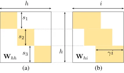
As a second way to sparsify the RNN cell, we propose to not provide all hidden dimensions with explicit access to each input dimension. In each row ofWhiwe limit the number of trainable

pa-rameters to a fraction γ ∈ ]0,1]. Practically, we choose to organize theγitrainable parameters in each row within a window that gradually moves from the first to the last input dimension, when ad-vancing in the hidden (i.e., row) dimension. Fur-thermore, we segment the hidden dimension of

h i

h _γi

Whh Whi

(a) (b)

s3 s2

s1

Figure 1: Predefined sparseness in hidden-to-hidden (Whh) and input-to-hidden (Whi)

matri-ces in RNNs. Trainable parameters (yellow) vs. zeros (white).

move the window ofγitrainable parameters dis-cretely per segment, as illustrated in Fig.1(b).

Because of the proposed practical arrangement of sparse and dense blocks in Whh and Whi,

the sparse RNN cell is equivalent to a composi-tion of smaller dense RNN’s operating in paral-lel on (partly) overlapping input data segments, with concatenation of the individual hidden states at the output. This will be illustrated at the end of Section5. As a result, fast libraries like CuDNN (Chetlur et al., 2014) can be used directly. Fur-ther research is required to investigate the poten-tial benefit in terms of speed and total cell capac-ity, of physically distributing computations for the individual dense recurrent cells.

Note that this is only possible because of the ini-tial requirement that the output dimensions are di-vided into disjoint segments. Whereas inputs can be shared entirely between different components, joining overlapping segments in theh dimension would need to be done within the cell, before ap-plying the gating and output non-linearities. This would make the proposed model less interesting for practical use.

We point out two special cases: (i) dense Whi

matrices (γ = 1) lead to N parallel RNNs that share the inputs but with separate contributions to the output, and (ii) organizingWhias a block ma-trix (e.g.,γ = 1/N forN same-length segments), leads to N isolated parallel RNNs. In the latter case, the reduction in trainable parameters is high-est, for a given number of segments, but there is no more influence from any input dimension in a given segment to output dimensions in non-cor-responding segments. We recommend option (i) as the most rational way to apply our ideas: the

sparse RNN output is a concatenation of individ-ual outputs of a number of RNN components con-nected in parallel, all sharing the entire input.

3.2 Language Modeling with Sparse RNNs

We apply predefined sparse RNNs to language modeling. Our baseline approach is the AWD-LSTM model introduced byMerity et al.(2017). The recurrent unit consists of a three-layer stacked LSTM (Long Short-Term Memory net-work (Hochreiter and Schmidhuber,1997)), with 400-dimensional inputs and outputs, and interme-diate hidden state sizes of 1150. Since the vo-cabulary contains only10k words, most trainable parameters are in the recurrent layer (20M out of a total of 24M). In order to cleanly measure the impact of predefined sparseness in the recurrent layer, we maintain the original word embedding layer dimensions, and sparsify the recurrent layer.3 In this example, we experiment with increasing dimensions in the recurrent layer while maintain-ing the number of trainable parameters, whereas in Section4.2we increase sparseness while main-taining dimensions.

Specifically, each LSTM layer is made sparse in such a way that the hidden dimension 1150 is increased by a factor 1.5 (chosenad hoc) to 1725, but the embedding dimensions and total number of parameters remain the same (within error margins from rounding to integer dimensions for the dense blocks). We use uniform segments. The number of parameters for the middle LSTM layer can be calculated as:4

# params. LSTM layer 2

= 4(hdid+h2d+ 2hd) (dense)

= 4N(hs Nγis+

h2

s

N2 + 2 hs

N) (sparse)

in which the first expression represents the gen-eral case (e.g., thedensecase has input and state sizes id = hd = 1150), and the second part is

the sparse case composed of N parallel LSTMs

3

Alternative models could be designed for comparison, with modifications in both the embedding and output layer. Straightforward ideas include an ensemble of smaller inde-pendent models, or a mixture-of-softmaxes output layer to combine hidden states of the parallel LSTM components, in-spired by (Yang et al.,2017).

4

This follows from an LSTM’s 4Whhand 4Whi

finetune test perplexity

(Merity et al.,2017) no 58.8

baseline no 58.8±0.3

sparse LSTM no 57.9±0.3

(Merity et al.,2017) yes 57.3

baseline yes 56.6±0.2

sparse LSTM yes 57.0±0.2

Table 1: Language modeling for PTB (mean±stdev).

with input size γis, and state size hs/N (with

is=hs = 1725).Denseandsparsevariants have

the same number of parameters for N = 3 and γ = 0.555. These values are obtained by identi-fying both expressions. Note that the equality in model parameters for the dense and sparse case holds only approximately due to rounding errors in(γis)and(hs/N).

Figure 1 displaysWhh andWhi for the mid-dle layer, which has close to11M parameters out of the total of 24M in the whole model. A dense model with hidden sizeh = 1725 would require 46M parameters, with 24M in the middle LSTM alone.

Given the strong hyperparameter dependence of the AWD-LSTM model, and the known is-sues in objectively evaluating language models (Melis et al., 2017), we decided to keep all hy-perparameters (i.e., dropout rates and optimiza-tion scheme) as in the implementaoptimiza-tion from Mer-ity et al. (2017)5, including the weight dropping with p = 0.5 in the sparse Whh matrices.

Ta-ble 1 shows the test perplexity on a processed version (Mikolov et al., 2010) of the Penn Tree-bank (PTB) (Marcus et al.,1993), both with and without the ‘finetune’ step6, displaying mean and standard deviation over 5 different runs. With-out finetuning, the sparse model consistently per-forms around 1 perplexity point better, whereas af-ter finetuning, the original remains slightly betaf-ter, although less consistently so over different ran-dom seeds. We observed that the sparse model overfits more strongly than the baseline, especially during the finetune step. We hypothesize that the

5_{Our implementation extends https://github.}

com/salesforce/awd-lstm-lm.

6_{The ‘finetune’ step indicates hot-starting the Averaged} Stochastic Gradient Descent optimization once more, after convergence in the initial optimization step (Merity et al., 2017).

regularization effect of a priori limiting interac-tions between dimensions does not compensate for the increased expressiveness of the model due to the larger hidden state size. Further experimen-tation, with tuned hyperparameters, is needed to determine the actual benefits of predefined sparse-ness, in terms of model size, resulting perplexity, and sensitivity to the choice of hyperparameters.

4 Sparse Word Embeddings

Given a vocabulary with V words, we want to construct vector representations of length k for each word such that the total number of parame-ters needed (i.e., non-zero entries), is smaller than k V. We introduce one way to do this based on word frequencies (Section4.1), and present part-of-speech tagging experiments (Section4.2).

4.1 Word-Frequency based Embedding Size

Predefined sparseness in word embeddings amounts to deciding which positions in the word embedding matrixE ∈ _RV×k _{should be fixed to}

zero, prior to training. We define the fraction of trainable entries in E as the embedding density δE. We hypothesize that rare words can be

represented with fewer parameters than frequent words, since they only appear in very specific contexts. This will be investigated experimentally in Section4.2. Word occurrence frequencies have a typical Zipfian nature (Manning et al., 2008), with many rare and few highly frequent terms. Thus, representing the long tail of rare terms with short embeddings should greatly reduce memory requirements.

In the case of a low desired embedding density δE, we want to save on the rare words, in terms of

assigning trainable parameters, and focus on the fewer more popular words. An exponential decay in the number of words that are assigned longer representations is one possible way to implement this. In other words, we propose to have the num-ber of words that receive a trainable parameter at dimensionjdecrease with a factorαj_{(α∈]0,1]).}

For a given fractionδE, the parameterαcan be

de-termined from requiring the total number of non-zero embedding parameters to amount to a given fractionδE of all parameters:

# embedding params.= k−1 X

j=0

αjV =δEk V

1 10 20 embedding dimension

1

20k

40k

vo

cab.

index

LF

HF

δE= 0.5 δE= 0.2 δE= 0.1

Figure 2: Visualization of sparse embedding ma-trices for different densities δE (with k = 20).

Colored region: non-zero entries. Rows represent word indices, sorted from least frequent (LF) to highly frequent (HF).

Figure2gives examples of embedding matrices with varying δE. For a vocabulary of 44k terms

and maximum embedding lengthk= 20, the den-sity δE = 0.2 leads to 25% of the words with

embedding length 1 (corresponding α = 0.75), only 7.6% with length of 10 or higher, and with the maximum length 20 for only the 192 most fre-quent terms. The particular configurations shown in Fig. 2 are used for the experiments in Sec-tion4.2.

In order to set a minimum embedding length for the rarest words, as well as for computational ef-ficiency, we note that this strategy can also be ap-plied onM bins of embedding dimensions, rather than per individual dimensions. The width of the first bin then indicates the minimum embed-ding length. Say bin m has widthκm (form = 0, . . . , M −1, andP

mκm =k). The

multiplica-tive decay factorαcan then be obtained by solving

δE = 1 k

M−1 X

m=0

κmαm, (1)

while numerically compensating for rounding er-rors in the numberV αm_{of words that are assigned}

trainable parameters in themth _bin.

4.2 Part-of-Speech Tagging Experiments

We now study the impact of sparseness in word embeddings, for a basic POS tagging model, and report results on the PTB Wall Street Journal data. We embed 43,815 terms in 20-dimensional space,

2 5 10 20

(average) embedding size 94

95 96

test

accuracy

(%)

dense sparse

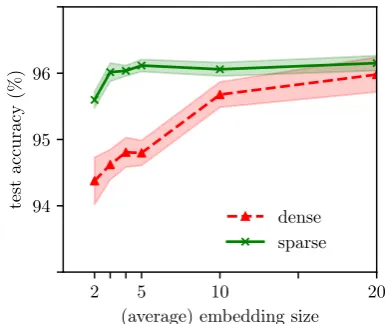
Figure 3: POS tagging accuracy on PTB data: dense (red) vs. sparse (green). X-axis: embedding sizekfor the dense case, and average embedding size (or20 δE) for the sparse case. Shaded bands

indicatestdevover 4 randomly seeded runs.

as input for a BiLSTM layer with hidden state size 10 for both forward and backward directions. The concatenated hidden states go into a fully connected layer with tanh non-linearity (down to dimension 10), followed by a softmax classi-fication layer with 49 outputs (i.e., the number of POS tags). The total number of parameters is 880k, of which 876k in the embedding layer. Although character-based models are known to outperform pure word embedding based models (Ling et al.,2015), we wanted to investigate the ef-fect of sparseness in word embeddings, rather than creating more competitive but larger or complex models, risking a smaller resolution in the effect of changing individual building blocks. To this end we also limited the dimensions, and hence the ex-pressiveness, of the recurrent layer.7 Our model is similar to but smaller than the ‘word lookup’ base-line byLing et al.(2015).

Figure 3 compares the accuracy for variable densitiesδE (fork= 20) vs. different embedding

sizes (withδE = 1). For easily comparing sparse

and dense models with the same number of em-bedding parameters, we scale δE, the x-axis for

the sparse case, to the average embedding size of 20δE.

7

Training models with shorter dense embeddings appeared more difficult. In order to make a fair comparison, we therefore tuned the models over a range of regularization hyperparameters, provided in Table2.

We observe that the sparse embedding layer allows lowering the number of parameters in

E down to a fraction of 15% of the original amount, with little impact on the effectiveness, provided E is sparsified rather than reduced in size. The reason for that is that with sparse 20-dimensional embeddings, the BiLSTM still re-ceives 20-dimensional inputs, from which a signif-icant subset only transmits signals from a small set of frequent terms. In the case of smaller dense em-beddings, information from all terms is uniformly present over fewer dimensions, and needs to be processed with fewer parameters at the encoder in-put.

Finally, we verify the validity of our hypothe-sis from Section4.1that frequent terms need to be embedded with more parameters than rare words. Indeed, one could argue in favor of the opposite strategy. It would be computationally more ef-ficient if the terms most often encountered had the smallest representation. Also, stop words are the most frequent ones but are said to carry little information content. However, Table 3 confirms our initial hypothesis. Applying the introduced strategy to sparsify embeddings on randomly or-dered words (‘no sorting’) leads to a significant de-crease in accuracy compared to the proposed sort-ing strategy (‘up’). When the most frequent words are encoded with the shortest embeddings (‘down’ in the table), the accuracy goes down even further.

5 Learning To Recite

From the language modeling experiments in Sec-tion 3.2, we hypothesized that an RNN layer be-comes more expressive, when the dense layer is replaced by a larger layer with predefined sparse-ness and the same number of model parameters. In this section, we design an experiment to further investigate this claim. One way of quantifying an RNN’s capacity is in measuring how much infor-mation it can memorize. We name our experimen-tal setuplearning to recite: we investigate to what extent dense vs. sparse models are able to learn an entire corpus by heart in order to recite it after-wards. We note that this toy problem could have interesting applications, such as the design of

neu-ral network components that keep entire texts or even knowledge bases available for later retrieval, encoded in the component’s weight matrices.8

5.1 Experimental Results

The initial model for ourlearning to recite exper-iment is the baseline language model used in Sec-tion 3.2(Merity et al., 2017), with the PTB data. We set all regularization parameters to zero, to fo-cus on memorizing the training data. During train-ing, we measure the ability of the model to cor-rectly predict the next token at every position in the training data, by selecting the token with high-est predicted probability. When the model reaches an accuracy of 100%, it is able to recite the entire training corpus. We propose the following opti-mization setup (tuned and tested on dense models with different sizes): minibatch SGD (batch size 20, momentum 0.9, and best initial learning rate among 5 or 10). An exponentially decaying learn-ing rate factor (0.97 every epoch) appeared more suitable for memorization than other learning rate scheduling strategies, and we report the highest accuracy in 150 epochs.

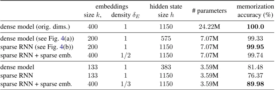
We compare the original model (in terms of net-work dimensions) with versions that have less pa-rameters, by either reducing the RNN hidden state size h or by sparsifying the RNN, and similarly for the embedding layer. For making the embed-ding matrix sparse,M = 10equal-sized segments are used (as in eq. 1). Table 4 lists the results. The dense model with the original dimensions has 24M parameters to memorize a sequence of in to-tal ‘only’930k tokens, and is able to do so. When the model’s embedding size and intermediate hid-den state size are halved, the number of parameters drops to7M, and the resulting model now makes 67 mistakes out of 10k predictions. If h is kept, but the recurrent layers are made sparse to yield the same number of parameters, only 5 mistakes are made for every 10k predictions. Making the embedding layer sparse as well introduces new er-rors. If the dimensions are further reduced to a third the original size, the memorization capacity goes down strongly, with less than 4M trainable parameters. In this case, sparsifying both the current and embedding layer yields the best re-sult, whereas the dense model works better than

hyperparameter value(s)

optimizer Adam (Kingma and Ba,2015)

learning rate 0.001

epochs 50

word level embedding dropout† [0.0, 0.1, 0.2] variational embedding dropout† [0.0, 0.1, 0.2, 0.4] DropConnect onWhh† [0.0, 0.2, 0.4]

batch size 20

Table 2: Hyperparameters for POS tagging model (†as introduced in (Merity et al.,2017)). A list indicates tuning over the given values was performed.

δE = 1.0 δE = 0.25 δE = 0.1

# params. (E; all) 876k;880k 219k;222k 88k ;91k

up 96.1±0.1 95.6±0.1

no sorting 96.0±0.3 94.3±0.4 93.0±0.3

down 89.8±2.2 90.6±0.5

Table 3: Impact of vocabulary sorting on POS accuracy with sparse embeddings: up vs. down (most fre-quent words get longest vs. shortest embeddings, resp.) or not sorted, for different embedding densities δE.

embeddings hidden state

# parameters memorization

sizek, densityδE sizeh accuracy (%)

dense model (orig. dims.) 400 1 1150 24.22M 100.0

dense model (see Fig.4(a)) 200 1 575 7.07M 99.33

sparse RNN (see Fig.4(b)) 200 1 1150 7.07M 99.95

sparse RNN + sparse emb. 400 1/2 1150 7.07M 99.74

dense model 133 1 383 3.59M 81.48

sparse RNN 133 1 1150 3.59M 76.37

sparse RNN + sparse emb. 400 1/3 1150 3.59M 89.98

Table 4: PTB train set memorization accuracies for dense models vs. models with predefined sparseness in recurrent and embedding layers with comparable number of parameters.

the model with sparse RNNs only. A possible ex-planation for that is the strong sparseness in the RNNs. For example, in the middle layer only 1 out of 10 recurrent connections is non-zero. In this case, increasing the size of the word embeddings (at least, for the frequent terms) could provide an alternative for the model to memorize parts of the data, or maybe it makes the optimization process more robust.

5.2 Visualization

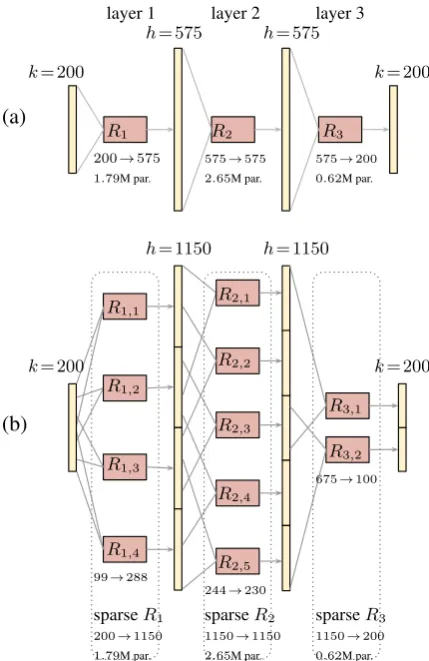
Finally, we provide an illustration of the high-level composition of the recurrent layers in two of

layer 1 layer 2 layer 3

(a)

k= 200

h= 575 h= 575

k= 200

R1 R2 R3

200→575 575→575 575→200 1.79M par. 2.65M par. 0.62M par.

(b)

k= 200

h= 1150 h= 1150

k= 200

R1,1

R1,2

R1,3

R1,4

R2,1

R2,2

R2,3

R2,4

R2,5

R3,1

R3,2

99→288

244→230

675→100

sparseR1 200→1150

sparseR2 1150→1150

sparseR3 1150→200 1.79M par. 2.65M par. 0.62M par.

Figure 4: Schematic overview of 3-layer stacked (a) dense vs. (b) sparse LSTMs with the same number of parameters (indicated with ‘par.’). Sparse layers are effectively composed of smaller dense LSTMs. ‘Ri,j’ indicates component j

within layeri, and ‘675→100’ indicates an LSTM compoment with input size 675 and output size 100.

6 Conclusion and Future Work

This paper introduces strategies to design word embedding layers and recurrent networks with predefined sparseness. Effective sparse word rep-resentations can be constructed by encoding less frequent terms with smaller embeddings and vice versa. A sparse recurrent neural network layer can be constructed by applying multiple smaller recur-rent cells in parallel, with partly overlapping in-puts and concatenated outin-puts.

The presented ideas can be applied to build models with larger representation sizes for a given number of parameters, as illustrated with a lan-guage modeling example. Alternatively, they can be used to reduce the number of parameters for given representation sizes, as investigated with a part-of-speech tagging model.

We introduced ideas on predefined sparseness in sequence models, as well as proof-of-concept ex-periments, and analysed the memorization capac-ity of sparse networks in the ‘learning to recite’ toy problem.

More elaborate experimentation is required to investigate the benefits of predefined sparseness on more competitive tasks and datasets in NLP. For example, language modeling results on the Penn Treebank rely on heavy regularization due to the small corpus. Follow-up work could there-fore investigate to what extent language models for large corpora can be trained with limited com-putational resources, based on predefined sparse-ness. Other ideas for future work include the use of predefined sparseness for pretraining word em-beddings, or other neural network components be-sides recurrent models, as well as their use in alter-native applications such as sequence-to-sequence tasks or in multi-task scenarios.

Acknowledgments

We thank the anonymous reviewers for their time and effort, and the valuable feedback.

References

Giannis Bekoulis, Johannes Deleu, Thomas Demeester, and Chris Develder. 2018. Joint entity recogni-tion and relarecogni-tion extracrecogni-tion as a multi-head selec-tion problem. Expert Systems with Applications, 114:34–45.

Ciprian Chelba, Tomas Mikolov, Mike Schuster, Qi Ge, Thorsten Brants, Phillipp Koehn, and Tony Robin-son. 2013. One billion word benchmark for measur-ing progress in statistical language modelmeasur-ing. Tech-nical report, Google.

Sharan Chetlur, Cliff Woolley, Philippe Vandermersch, Jonathan Cohen, John Tran, Bryan Catanzaro, and Evan Shelhamer. 2014. cuDNN: Efficient primitives for deep learning.arXiv:1410.0759.

Junyoung Chung, C¸ alar G¨ulc¸ehre, Kyunghyun Cho, and Yoshua Bengio. 2014. Empirical evaluation of gated recurrent neural networks on sequence model-ing. arXiv:1412.3555. Deep Learning workshop at NIPS 2014.

Ian Goodfellow, Yoshua Bengio, and Aaron Courville. 2016. Deep Learning. MIT Press. http://www.

deeplearningbook.org.

Song Han, Huizi Mao, and William J. Dally. 2016. Deep compression: Compressing deep neural net-works with pruning, trained quantization and Huff-man coding. InProc. 4th International Conference on Learning Representations (ICLR 2016).

Song Han, Jeff Pool, John Tran, and William J. Dally. 2015. Learning Both Weights and Connections for Efficient Neural Networks. In Proc. 28th Interna-tional Conference on Neural Information Processing Systems (NIPS 2015), NIPS’15, pages 1135–1143.

Kazuma Hashimoto, Caiming Xiong, Yoshimasa Tsu-ruoka, and Richard Socher. 2017. A joint many-task model: Growing a neural network for multiple nlp tasks. In Proc. Conference on Empirical Methods in Natural Language Processing (EMNLP), pages 1923–1933.

Sepp Hochreiter and J¨urgen Schmidhuber. 1997. Long short-term memory. Neural computation, 9(8):1735–1780.

Max Jaderberg, Andrea Vedaldi, and Andrew Zisser-man. 2014. Speeding up convolutional neural net-works with low rank expansions. In Proc. 27th British Machine Vision Conference (BMVC 2014). ArXiv: 1405.3866.

Nal Kalchbrenner, Erich Elsen, Karen Simonyan, Seb Noury, Norman Casagrande, Edward Lockhart, Flo-rian Stimberg, A¨aron van den Oord, Sander Diele-man, and Koray Kavukcuoglu. 2018. Efficient neu-ral audio synthesis. ArXiv: 1802.08435.

Diederik Kingma and Jimmy Ba. 2015. Adam: A method for stochastic optimization. In Interna-tional Conference on Learning Representations, San Diego, USA.

V. Lebedev and V. Lempitsky. 2016. Fast ConvNets using group-wise brain damage. InProc. 29th IEEE Conference on Computer Vision and Pattern Recog-nition (CVPR 2016), pages 2554–2564.

Wang Ling, Chris Dyer, Alan W Black, Isabel Tran-coso, Ramon Fermandez, Silvio Amir, Luis Marujo, and Tiago Luis. 2015. Finding function in form: Compositional character models for open vocabu-lary word representation. InProceedings of the 2015 Conference on Empirical Methods in Natural Lan-guage Processing, pages 1520–1530, Lisbon, Portu-gal. Association for Computational Linguistics.

Baoyuan Liu, Min Wang, H. Foroosh, M. Tappen, and M. Penksy. 2015. Sparse convolutional neural net-works. InProc. 28th IEEE Conference on Computer Vision and Pattern Recognition (CVPR 2015), pages 806–814.

Zhiyun Lu, Vikas Sindhwani, and Tara N. Sainath. 2016. Learning compact recurrent neural networks. In Proc. 41st IEEE International Conference on Acoustics, Speech and Signal Processing (ICASSP 2016).

Christopher D. Manning, Prabhakar Raghavan, and Hinrich Sch¨utze. 2008. Introduction to Information Retrieval. Cambridge University Press, New York, NY, USA.

Mitchell P. Marcus, Beatrice Santorini, and Mary Ann Marcinkiewicz. 1993. Building a large annotated corpus of english: The penn treebank. Computa-tional Linguistics, 19(2):313–330.

Gbor Melis, Chris Dyer, and Phil Blunsom. 2017. On the state of the art of evaluation in neural language models. In Proc. 6th International Conference on Learning Representations (ICLR 2017).

Stephen Merity, Nitish Shirish Keskar, and Richard Socher. 2017. Regularizing and optimizing LSTM language models.arXiv:1708.02182.

Tomas Mikolov, Martin Karafit, Luks Burget, Jan Cer-nock, and Sanjeev Khudanpur. 2010. Recurrent neural network based language model. In INTER-SPEECH, pages 1045–1048. ISCA.

Makoto Miwa and Mohit Bansal. 2016. End-to-end relation extraction using LSTMs on sequences and tree structures. InProc. 54th Annual Meeting of the Association for Computational Linguistics, pages 1105–1116.

Dmitry Molchanov, Arsenii Ashukha, and Dmitry Vetrov. 2017. Variational dropout sparsifies deep neural networks. In Proc. 35th International Con-ference on Machine Learning (ICML 2017). ArXiv: 1701.05369.

Sharan Narang, Erich Elsen, Gregory Diamos, and Shubho Sengupta. 2017. Exploring sparsity in recurrent neural networks. In Proc. 5th Inter-national Conference on Learning Representations (ICLR 2017).

Adam Paszke, Sam Gross, Soumith Chintala, Gre-gory Chanan, Edward Yang, Zachary DeVito, Zem-ing Lin, Alban Desmaison, Luca Antiga, and Adam Lerer. 2017. Automatic differentiation in pytorch. In Proceedings of the Workshop on The future of gradient-based machine learning software and tech-niques, co-located with the 31st Annual Conference on Neural Information Processing Systems (NIPS 2017).

Noam Shazeer, Azalia Mirhoseini, Krzysztof Maziarz, Andy Davis, Quoc Le, Geoffrey Hinton, and Jeff Dean. 2017. Outrageously large neural networks: The sparsely-gated mixture-of-experts layer. In

Proc. International Conference on Learning Repre-sentations (ICLR).

Li Wan, Matthew Zeiler, Sixin Zhang, Yann LeCun, and Rob Fergus. 2013. Regularization of neural net-works using dropconnect. In Proc. 30th Interna-tional Conference on InternaInterna-tional Conference on Machine Learning (ICML 2013), pages III–1058– III–1066, Atlanta, GA, USA.

Dong Wang, Qiang Zhou, and Amir Hussain. 2016. Deep and sparse learning in speech and language processing: An overview. In Proc. 8th Interna-tional Conference on (BICS2016), pages 171–183. Springer, Cham.

Wei Wen, Chunpeng Wu, Yandan Wang, Yiran Chen, and Hai Li. 2016. Learning structured sparsity in deep neural networks. In Proc. 30th Interna-tional Conference on Neural Information Processing Systems (NIPS 2016), NIPS’16, pages 2082–2090, USA.