Computational Analysis of Flow between two Parallel Plates

(1)

©IJRASET: All Rights are Reserved

912

Computational Analysis of Flow between two

Parallel Plates

Dinesh Kumar1, Kapil Kumar2 1

Assistant Professor Department of Mechanical Engineering, Institute of Technology Gopeshwar, Uttarakhand, India

2

Research Scholar, Department of Mechanical Engineering, Uttarakhand Technical University Dehradun, India

Abstract: Computational fluid dynamics (CFD) is a branch of fluid mechanics that uses numerical methods and algorithms to solve and analyze problems that involve fluid flows. Computers are used to perform the calculations required to simulate the interaction of liquids and gases with surfaces defined by boundary conditions. With Modern Engineers apply both experimental and CFD analysis, and the two complement to each other.

Example: Engineers may obtain global properties, such as lift, drag, pressure drop, or power, experimentally, but use CFD to obtain details about the flow field, such as shear stresses, velocity and pressure profiles, and flow streamlines. In addition experimental data are often used to validate CFD solution by matching the computationally and experimentally determined global quantities. CFD is then employed to shorten the design cycle through carefully controlled parametric studies, thereby reducing the required amount of experimental testing.

In our present discussion we merely scratch the surface of this exciting field. Our goal is to present the fundamentals of CFD from a user’s point of view, providing guidelines about how to generate a grid, how to specify boundary conditions, and how to determine if the computer output is physically meaningful.

There are two fundamental approaches to design and analysis of engineering systems that involve fluid flow.

1) Experimental: It involves construction of model that are tested in wind tunnel or other facilities. However, in many cases in real-life engineering, the equations are either not known or too difficult to solve; often times experimentation is the only method of obtaining reliable information.

2) Calculation: It involves solution of differential equations, either

a. Analytically: In this method the equations are solved analytically. Unfortunately, most differential equations encountered in fluid mechanics are very difficult to solve and often require the aid of a computer.

b. Computationally: In this method the equations are solved with the help of computers. Using CFD software we can build a ‘virtual prototype’ of the system or device that we wish to analyze and then apply real world physics and chemistry to the model and then software will provide images and data, which predict the performance of that design.

Keywords: Computational fluid dynamics, Taylor’s Series Truncation, Discretization Method, Grid Generation, Convergence Program.

I. INTRODUCTION

Computational fluid dynamics (CFD) is the science of predicting fluid flow, heat transfer, mass transfer, chemical reactions, and related phenomena by solving the mathematical equations which govern these processes using a numerical process.

The result of CFD analyses is relevant engineering data used in:

1) Conceptual studies of new designs.

2) Detailed product development.

3) Troubleshooting.

4) Redesign

5) Reduces the total effort required in the laboratory.

(2)

[image:2.612.200.418.131.290.2]

913

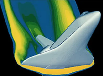
CFD made possible by the advent of digital computer and advancing with improvements of computer resources. The broad area of CFD leads to many different closely related but nevertheless specialized technology areas. These include: grid generation, flow field discretization algorithms, efficient solution of large systems of equations, massive data storage and transmission technology methods, computational flow visualization

Fig 1 A computer simulation of high velocity air flow around

II. BENEFITS OF CFD

Using CFD, you can build a computational model that represents a system or device that you want to study. Then you apply the fluid flow physics and chemistry to this virtual prototype, and the software will output a prediction of the fluid dynamics and related physical phenomena. There are three compelling reasons to use CFD software: insight, foresight, and efficiency.

A. Insight

If you have a device or system design which is difficult to prototype or test through experimentation, CFD analysis enables you to virtually crawl inside your design and see how it performs. There are many phenomena that you can witness through CFD, which wouldn't be visible through any other means. CFD gives you a deeper insight into your designs.

Fig. 2 Simulation of flow over a male elite swimmer gliding under water

B. Foresight

Because CFD is a tool for predicting what will happen under a given set of circumstances, it can quickly answer many 'what if?' questions. You provide a set of boundary conditions, and the software gives you outcomes. In a short time, you can predict how your design will perform, and test many variations until you arrive at an optimal result. All of this can be done before physical prototyping and testing.

C. Efficiency

[image:2.612.211.399.436.560.2]

(3)

914

III. ADVANTAGES OF CFD

A. Relatively Low Cost

1) Using physical experiments and tests to get essential engineering data for design can be expensive

2) CFD simulations are relatively inexpensive, and costs are likely t0 decrease as computers become more powerful.

B. Speed

1) CFD simulations can be executed in a short period of time.

2) Quick turnaround means engineering data can be introduced early in the design process.

C. Ability to Simulate Real Conditions

1) Many flow and heat transfer processes cannot be (easily) tested, e.g. hypersonic flow.

2) CFD provides the ability to theoretically simulate any physical Condition.

D. Ability to Simulate Ideal Conditions

1) CFD allows great control over the physical process, and provides the ability to isolate specific phenomena for study.

2) Example: a heat transfer process can be idealized with adiabatic, constant heat flux, or constant temperature boundaries.

IV. APPLICATIONS OF CFD

Flow and heat transfer in industrial processes (boilers, heat exchangers, combustion equipment, pumps, blowers, piping, etc.). Aerodynamics of ground vehicles, aircraft, missiles

Film coating, thermoforming in material processing applications. Flow and heat transfer in propulsion and power generation systems. Ventilation, heating, and cooling flows in buildings

Chemical vapor deposition (CVD) for integrated circuit manufacturing. Heat transfer for electronics packaging applications.

And many, many more!

V. LIMITATIONS OF CFD

A. Physical Models

1) CFD solutions rely upon physical models of real world processes (e.g. turbulence, compressibility, chemistry, multiphase flow,

etc.).

2) The CFD solutions can only be as accurate as the physical models on which they are based.

B. Numerical Errors

1) Solving equations on a computer invariably introduces numerical errors.

2)Round-Off Error: due to finite word size available on the computer. Round-off errors will always exist (though they can be small in most cases).

[image:3.612.168.416.583.707.2]

3)Truncation Error: due to approximations in the numerical models. Truncation errors will go to zero as the grid is refined. Mesh refinement is one way to deal with truncation error.

(4)

915

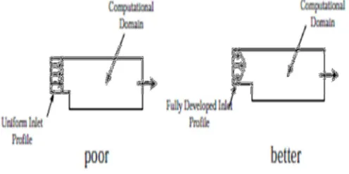
As with physical models, the accuracy of the CFD solution is only as good as the initial/boundary conditions provided to the numerical model.

Example: flow in a duct with sudden expansion. If flow is supplied to domain by a pipe, you should use a fully-developed profile for velocity rather than assume uniform conditions.

VI. CFD PROCESS

There are essentially three stages to every CFD simulation process: preprocessing, solving and post processing.

A. Preprocessing

This is the first step in building and analyzing a flow model. It includes building the model within a computer-aided design (CAD) package, creating and applying a suitable computational mesh, and entering the flow boundary conditions and fluid materials properties.

A computational domain is chosen, and a grid is generated.

Boundary conditions are specified on each edge of computational domain.

Type of fluid is specified , along with fluid properties(temperature , density , viscosity etc.)

Starting values for all flow field variables are specified for each grid. These are called initial conditions

1) Solving: The simulation is started and equations aresolved iteratively as steady state or transient. Using the equations iterations are done to converge on a final solution.

2) Post Processing: This is the final step in CFD analysis,and it involves the organization and interpretation of the predicted flow data and the production of CFD images and animations. Is used for analysis and visualization of the resulting solution.

B. Governing Equations in CFD Continuity Equation:

∂ ρ ∂ ρ u ∂ ρ v ∂ ρ w

0

∂ t ∂ x ∂ y ∂ z

Navier -Stokes Equations:

∂u ∂u ∂u ∂u ∂pˆ ∂2u ∂2u ∂2u

ρ ρu ρv ρw

∂t ∂x ∂y ∂z ∂x

2 2 2

∂x ∂y ∂z

Even though many methods are there to discretize a given grid but we will restrict our discussion to FDM.

The idea of FDM is to approximate the partial derivative in a physical equation by “differences” between nodal values a finite difference apart-a sort of numerical calculus.

The basic partial differential equation is thus replaced by a set of algebraic equation for the nodal values.

(5)

916

1) Structured Grid: Single structured grid.

a) i j k indexing to locate neighboring cells.

b) Grid lines must pass all through domain.

Obviously can’t be used for very complicated geometries military application. Since then, his "linear programming" techniques and their descendents were

Fig.5 - structured grid

2) Unstructured Grids: Different types of hexahedral grids.

a) Unstructured.

b) The mesh has no logical representation.

Fig.6 8-un structured grid

3) Boundary Conditions: When solving the Navier-Stokes equation and continuity equation, appropriate initial conditions and boundary conditions need to be applied.

(6)

917

In the example here, a no-slip boundary condition is applied at the solid wall.

Fig.8 no-slip boundary condition

(7)

918

4) CFD Program

#include<stdio.h> #include<conio.h> #include<math.h> void main() {

float u[100][100],v[100][100],vort[100][100],stream[100][100],KU[100][100],LU[100][100]; float L1[100][100],L2[100][100],K[100][100],KE[100][100],KF[100][100],VORTnew[100][100]; float STREAMnew[100][100],Vnew[100][100],KFU[100][100],KGU[100][100],Unew[100][100]; float KUnew[100][100],LUnew[100][100],L1new[100][100],L2new[100][100],Knew[100][100]; int E1[100][100],E2[100][100],E3[100][100],E4[100][100];

int dx=1,dy=1,m=10,n=10; int dt=1,i,j,U=2,flag=0; clrscr();

for(i=1;i<=m;i++) {

for(j=1;j<=n;j++) {

u[i][j]=1; Unew[i][j]=1; v[i][j]=1; Vnew[i][j]=1; E1[i][j]=1; E2[i][j]=1; E3[i][j]=1; E4[i][j]=1; vort[i][j]=1; VORTnew[i][j]=1; stream[i][j]=1; STREAMnew[i][j]=1; }

}

/*initiallisation of boundary condition */ /*for u and v */

/*at 1*/

for(j=2;j<=n-1;j++) {

u[1][j]=U; v[1][j]=0; }

/*at 2*/

for(i=1;i<=m;i++) {

u[i][n]=0; v[i][n]=0; }

/*at 4*/

for(i=1;i<=m;i++) {

u[i][1]=0; v[i][1]=0; }

/* for stream function*/ /*at 1*/

for(j=2;j<=n-1;j++) {

(8)

919

}

/* at 2*/

for(i=1;i<=m;i++) {

stream[i][n]=((4*stream[i][n-1])-stream[i][n-2])/3; }

/*at 4*/

for(i=1;i<=m;i++) {

stream[i][1]=((4*stream[i][2])-stream[i][3])/3; }

/*at 3*/

for(j=2;j<=n-1;j++) {

stream[m][j]=(2*dx*v[m-2][j])+(4*stream[m-1][j])-(3*stream[m-2][j]); }

/* B.C for u and v at 3*/ /* for v*/

for(j=2;j<=n-1;j++) {

v[m][j] = ((4*stream[m-1][j])-(stream[m-2][j])-(3*stream[m][j]))/(2*dx); }

/*for u*/

for(j=2;j<=(n/2);j++) {

KU[m][j]=((-stream[m][j+2])+(4*stream[m][j+1])-(3*stream[m][j]))/(2*dx); }

for(j=((n/2)+1);j<=n-1;j++) {

KU[m][j]=0; }

for(j=n-1;j>=(n/2);j--) {

LU[m][j]=((3*stream[m][j])-(4*stream[m][j-1])+(stream[m][j-2]))/(2*dx); }

for(j=((n/2)-1);j>=2;j--) {

LU[m][j]=0; }

for(j=2;j<=n-1;j++) {

u[m][j]=KU[m][j]+LU[m][j]; }

/*B.C for vorticity*/ /* at 1 */

for(j=2;j<=n-1;j++) {

vort[1][j]=((stream[1][j]-stream[2][j])*2)/(dx*dx); }

/*at 2*/

for(i=1;i<=m;i++) {

vort[i][n]=((stream[i][n]-stream[i][n-1])*2)/(dx*dx); }

/*at 4*/

(9)

920

vort[i][1]=((stream[i][1]-stream[i][2])*2)/(dx*dx);

} /*at 3*/

for(j=n-1;j>=(n/2);j--) {

L1[m][j]=((2*stream[m][j])-(5*stream[m][j-1])+(4*stream[m][j-2])-(stream[m][j-3]))/(dx*dx); }

for(j=((n/2)-1);j>=2;j--) {

L1[m][j]=0; }

for(j=2;j<=(n/2);j++) {

L2[m][j]=((-stream[m][j+3])+(4*stream[m][j+2])-(5*stream[m][j+1])+(2*stream[m][j]))/(dx*dx); }

for(j=((n/2)+1);j<=n-1;j++) {

L2[m][j]=0; }

for(j=2;j<=n-1;j++) {

K[m][j]=((2*stream[m][j])-(5*stream[m-1][j])+(4*stream[m-2][j])-(stream[m-3][j]))/(dx*dx); }

for(j=2;j<=n-1;j++) {

vort[m][j]=-K[m][j]-L1[m][j]-L2[m][j]; }

for(j=2;j<=n-1;j++) {

KE[i][j]=(((vort[i+1][j]-(2*vort[i][j])+vort[i-1][j])/(dx*dx))+((vort[i][j+1]-(2*vort[i][j])+vort[i][j-1])/(dy*dy)))*(v[i][j]*dt); }

}

for(i=2;i<=m-1;i++) {

for(j=2;j<=n-1;j++) {

KF[i][j]=(u[i][j]*dt)*((vort[i+1][j]-vort[i-1][j])/(2*dx))+((v[i][j]*dt)*((vort[i][j+1]-vort[i][j-1])/(2*dy))); }

}

for(i=2;i<=m-1;i++) {

for(j=2;j<=n-1;j++) {

VORTnew[i][j]=KE[i][j]-KF[i][j]+vort[i][j]; }

}

/* for new stream*/ for(i=2;i<=m-1;i++) {

for(j=2;j<=n-1;j++) {

(10)

921

}

/* for new V*/ for(i=2;i<=m-1;i++) {

for(j=2;j<=n-1;j++) {

Vnew[i][j]=(STREAMnew[i-1][j]-STREAMnew[i+1][j])/(2*dx); }

}

/*for new U*/ for(i=2;i<=(m/2);i++) {

for(j=2;j<=n-1;j++) {

KFU[i][j]=((Vnew[i][j+1])-(Vnew[i][j-1])-(u[i+2][j])+(4*u[i+1][j]))/3; }

}

for(i=((m/2)+1);i<=m-1;i++) {

for(j=2;j<=n-1;j++) {

KFU[i][j]=0; }

}

for(i=m-1;i>=(m/2);i--) {

for(j=2;j<=n-1;j++) {

KGU[i][j]=((Vnew[i][j-1])-Vnew[i][j+1]+(4*u[i-1][j])-(u[i-2][j]))/3; }

}

for(i=((m/2)-1);i>=2;i--) {

for(j=2;j<=n-1;j++) {

KGU[i][j]=0; }

}

for(i=2;i<=m-1;i++) {

for(j=2;j<=n-1;j++) {

Unew[i][j]=KFU[i][j]+KGU[i][j]; }

}

/* initialisation of new B.C*/

/*for Unew and Vnew*/ /*at 1*/

for(j=2;j<=n-1;j++) {

Unew[1][j]=1; Vnew[1][j]=0; }

/*at 2*/

(11)

922

Unew[i][n]=0;

Vnew[i][n]=0; }

/*at 4*/

for(i=1;i<=m;i++) {

Unew[i][1]=0; Vnew[i][1]=0; }

/* B.C for new stream function*/ /*at 1*/

for(j=2;j<=n-1;j++) {

STREAMnew[1][j]=((4*STREAMnew[2][j])-STREAMnew[3][j])/3; }

/*at 2*/

for(i=1;i<=m;i++) {

STREAMnew[i][n]=((4*STREAMnew[i][n-1])-(STREAMnew[i][n-2]))/3; }

/*at 4*/

for(i=1;i<=m;i++) {

STREAMnew[i][1]=((4*STREAMnew[i][2])-(STREAMnew[i][3]))/3; }

/*at 3*/

for(j=2;j<=n-1;j++) {

STREAMnew[m][j]=(2*dx*Vnew[m-2][j])+(4*STREAMnew[m-1][j])-(3*STREAMnew[m-2][j]); }

/* Vnew and Unew at 3*/ /*Vnew at 3*/

for(j=2;j<=n-1;j++) {

Vnew[m][j]=((4*STREAMnew[m-1][j])-(STREAMnew[m-2][j])-(3*STREAMnew[m][j]))/(2*dx); }

/*Unew at 3*/ for(j=2;j<=(n/2);j++) {

KUnew[m][j]=((-STREAMnew[m][j+2])+(4*STREAMnew[m][j+1])-(3*STREAMnew[m][j]))/(2*dx); }

for(j=((n/2)+1);j<=n-1;j++) {

KUnew[m][j]=0; }

for(j=n-1;j>=(n/2);j--) {

LUnew[m][j]=((3*STREAMnew[m][j])-(4*STREAMnew[m][j-1])+(STREAMnew[m][j-2]))/(2*dx); }

for(j=((n/2)-1);j>=2;j--) {

LUnew[m][j]=0; }

for(j=2;j<=n-1;j++) {

(12)

923

}

/*B.C for new vorticity*/ /*at 1*/

for(j=2;j<=n-1;j++) {

VORTnew[1][j]=((STREAMnew[1][j]-STREAMnew[2][j])*2)/(dx*dx); }

/*at 2*/

for(i=1;i<=m;i++) {

VORTnew[i][n]=((STREAMnew[i][n]-STREAMnew[i][n-1])*2)/(dx*dx); }

/*at 4*/

for(i=1;i<=m;i++) {

VORTnew[i][1]=((STREAMnew[i][1]-STREAMnew[i][2])*2)/(dx*dx); }

/*at 3*/

for(j=n-1;j>=(n/2);j--) {

L1new[m][j]=((2*STREAMnew[m][j])-(5*STREAMnew[m][j-1])+(4*STREAMnew[m][j-2])-(STREAMnew[m][j-3]))/(dx*dx);

}

for(j=((n/2)-1);j>=2;j--) {

L1new[m][j]=0; }

for(j=2;j<=(n/2);j++) {

L2new[m][j]=((-STREAMnew[m][j+3])+(4*STREAMnew[m][j+2])-(5*STREAMnew[m][j+1])+(2*STREAMnew[m][j]))/(dx*dx);

}

for(j=((n/2)+1);j<=n-1;j++) {

L2new[m][j]=0; }

for(j=2;j<=n-1;j++) {

Knew[m][j]=((2*STREAMnew[m][j])-(5*STREAMnew[m-1][j])+(4*STREAMnew[m-2][j])-(STREAMnew[m-3][j]))/(dx*dx);

}

for(j=2;j<=n-1;j++) {

VORTnew[m][j]=((-Knew[m][j])-(L1[m][j])-(L2[m][j])); }

for(i=1;i<=m;i++) {

for(j=1;j<=n;j++) {

E1[i][j]=abs(VORTnew[i][j]-vort[i][j]); E2[i][j]=abs(STREAMnew[i][j]-stream[i][j]); E3[i][j]=abs(Unew[i][j]-u[i][j]);

E4[i][j]=abs(Vnew[i][j]-v[i][j]); }

(13)

924

for(i=1;i<=m;i++)

{

for(j=1;j<=n;j++) {

if(E1[i][j]<=0.01&&E2[i][j]<=0.01&&E3[i][j]<=0.01&&E4[i][j]<=0.01) {

flag=0; } else { flag=1; } } }

if(flag==0) {

printf("i, j, u, v, vortstream"); printf("\n");

for(i=1;i<=m;i++) {

for(j=1;j<=n;j++) {

printf("%d %d %f %f %f %f",i,j,u[i][j],v[i][j],vort[i][j],stream[i][j]); printf("\n");

} } }

else {

for(i=1;i<=m;i++) {

for(j=1;j<=n;j++) {

vort[i][j]=VORTnew[i][j]; stream[i][j]=STREAMnew[i][j]; u[i][j]=Unew[i][j];

v[i][j]=Vnew[i][j]; }

} goto next; }

/* printf("i j "); printf("\n"); for(i=1;i<=2;i++) {

for(j=1;j<=10;j++) {

printf("%d %d %f",i,j,VORTnew[i][j]); printf("\n");

(14)

925

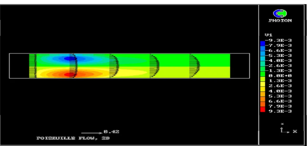
[image:14.612.74.578.120.360.2]

VII. RESULT

Fig 9 shows the CFD analysis image of flow between two parallel plates. The arrows in between the plate show the distribution of velocity. The different colures shows different flow speed mention in right side of figure.

Fig.9 CFD analysis

REFERENCES

[1] Anglart, H., and Podowski, M. Z. 2002. Fluid mechanics of Taylor bubbles and slug flows in vertical channels. Nuclear science and engineering, 140, 165-171. [2] Baker, O. 1954. Simultaneous flow of oil and gas. Oil & Gas Journal, 53, 184-195.

[3] Cook, M., and Behnia, M. 2001. Bubble motion during inclined intermittent flow. Int. J. of Heat and Fluid Flow, 22, 543-551. [4] Frank, T. 2003. Numerical simulations of multiphase flows using CFX-5. CFX Users conference, Garmisch-Partenkirchen, Germany.

[5] Hope, C. B. 1990. The development of a water soluble photochromic dye tracing technique and its application to two phase flow. PhD thesis, Imperial College of Science, Technology and Medicine, London.

[6] Ishii M. 1990. Two-fluid model for two-phase flow. Multiphase Science and Technology, 5, Edited by G. F. Hewitt, J. M. Delhaye, N. Zuber, Hemisphere Publishing Corporation, 1-64.

[7] Issa, R. I., and Tang, I. F. 1990. Modelling of vertical gas-liquid slug flow in pipes. Proc. Symp. On Advances in Gas-Liquid flows, Dallas. [8] Lun, I., Calay, R. K., and Holdo, A. E. 1996. Modelling two-phase flows using CFD. Applied Energy, 53, 299-314.

[9] Manfield, P. D. 2000. Experimental, computational and analytical studies of slug flow. PhD thesis, Imperial College of Science, Technology and Medicine, London.