WCE 2012 ISBN: 978-988-19252-1-3

TABLE I

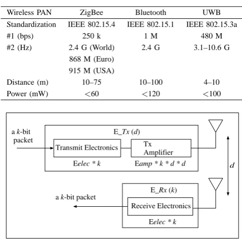
WIRELESS COMMUNICATION STANDARDS FOR THE HOME.

Wireless PAN ZigBee Bluetooth UWB

Standardization IEEE 802.15.4 IEEE 802.15.1 IEEE 802.15.3a

#1 (bps) 250 k 1 M 480 M

#2 (Hz) 2.4 G (World) 2.4 G 3.1–10.6 G

868 M (Euro) 915 M (USA)

Distance (m) 10–75 10–100 4–10

Power (mW) <60 <120 <100

a k-bit packet

Transmit Electronics Tx_Amplifier

Eamp * k * d * d

Eelec * k

E_Tx (d)

Receive Electronics

Eelec * k

E_Rx (k) a k-bit packet

d

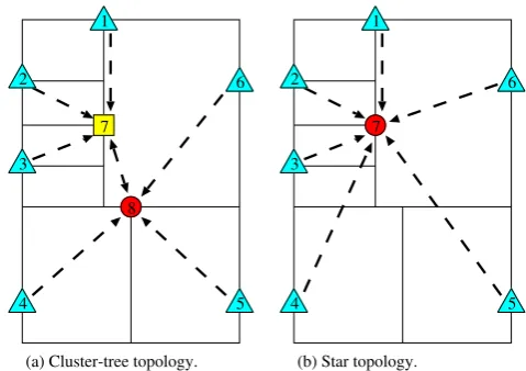
Fig. 2. The radio model for power consumption in a sensor node.

B. Power consumption in a sensor node

Fig 2 shows the radio model for the power consumption of transmitting and receiving a message in a sensor node [6]. To transmit a k-bit message within a distance d meters using the model, the radio of power (ET x(k, d)) expends in

the following Equation 1:

ET x(k, d) = ET x₋elec(k) +ET x₋amp(k, d)

= Eelec×k+Eamp×k×d2 (1)

To receive this message, the radio of power (ERx(k))

expends in the following Equation 2:

ERx(k) = ERx₋elec(k)

= Eelec×k (2)

whereEelec=ET x−elec=ERx−elec. In this paper, it is also

assumed the radio dissipates Eelec = 50 nJ/bit to run the

transmitter or receiver circuitry andEamp= 100 pJ/bit/m2.

III. ZIGBEE

In this section, an overview, the devices, and the topologies of ZigBee are described.

A. An Overview of ZigBee

ZigBee [4],[5],[13] is one of the standards for wireless communication at close range, which are used for applica-tions of the sensor network. The communication speed of ZigBee is faster than that of Bluetooth. The distance for data transmission of ZigBee is shorter than that of Bluetooth. The ZigBee has the features of low power-consumption, low cost of hardware, high reliability, and so on. The ZigBee drives about a few years by an AA or LR6 sized alkaline-battery. The speed of data transmission is utmost 250 kbps and the distance of the transmission is about maximum 75 meters. More than 65,000 devices are allowed to connect with each

(a) Star topology

(b) Cluster-tree topology

(c) Mesh topology

ZigBee Coordinator ZigBee Routers

ZigBee End-devices Wireless Connection

Fig. 3. Topologies for ZigBee.

other in the network. The network topologies have a star, a cluster-tree, and a mesh. A routing protocol of ZigBee is used the Ad Hoc On-Demand Distance Vector (AODV) Routing [21].

B. Devices of ZigBee

The ZigBee has a physical and logical device. The physical device based on the platform of hardware is classifies as two types: FFD (Full Function Device) and RFD (Reduced Function Device). The logical device based on the roles is classifies as three types: a ZigBee coordinator, a ZigBee router, and a ZigBee end-device as follows:

• ZigBee coordinator: There exists only one device in the ZigBee network. The device is to start on building the network. This network is built by connecting the coor-dinator with some devices on demand, which participate in the network.

• ZigBee router: This device may connect with the ZigBee coordinator, some of the other ZigBee routers, and some ZigBee end-devices, which have already joined in the network. The router transmits messages for multihop routing. The router also has a role of connecting some devices which are just participating in the network.

1

3

0

2 4

1

3

0

2 4 5

1

3

0

6 4

5 2

7

(a) Star topology (b) Cluster-tree topology

(c) Mesh topology

ZigBee Coordinator ZigBee Routers ZigBee End-devices

Fig. 4. Topologies for the simulation 1.

C. Topologies of ZigBee

Fig 3 shows the topologies for ZigBee. There are three types of topology: a star, a cluster-tree, and a mesh as follows.

• Star: This is a star topology which the ZigBee coordina-tor is connected with ZigBee end-devices. The topology is also the simplest one (Fig 3a).

• Cluster-tree: This is a tree topology which the ZigBee coordinator is as a root and also the ZigBee routers and the ZigBee end-devices are as leaves. The router makes the star topology, which the router itself is as a center and also it connects with the end-devices (Fig 3b).

• Mesh: This is a mesh topology which the ZigBee coor-dinator and the ZigBee routers are connected with each other. Each end-device is connected with the coordinator or the router (Fig 3c).

IV. EVALUATION

In this section, simulation methods and the results are presented.

A. Methods

In this here, to evaluate the power consumption on the topologies in Figs 4 and 5 as described in Subsection II-A, we conducted simulation studies.

We assumed the communication standard as ZigBee as described in Subsection II-A and in Section III. We also assumed that the information on sensing by nodes as end-devices were sent to a node as the coordinator directly or relaying some nodes as the routers, i.e., one way communi-cation from end-devices and/or relaying some routers to the coordinator.

For the information as packets transmission, we used the NS-2 simulator [22]. The size of a packet was used for 1000 bytes. The amount of packets obtained in the simulations was converted into that of the power consumption by using the model of a sensor node as described in Subsection II-B. The details for simulations are as follows:

Simulation 1: To evaluate the power consumption as the basis for this, we used the topologies in Fig 4. The distance of one hop between nodes was the same on the topologies.

(a) Cluster-tree topology. (b) Star topology. 1

2

3

4 5

6

7

8

1

2

3

4 5

6

7

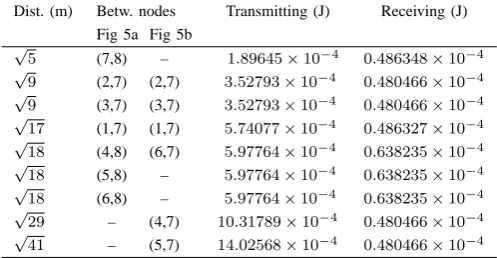
Fig. 5. Deployment of sensor nodes in the home for the simulation 2.

The power consumption on each topoloy was evaluated by comparing them. Note that the following parameters were the same in all simulations: 20 meters as the distance for one hop, four steps on running in a simulation, two seconds in each step for the communication time, and the performance of each node. The details in the simulations were as follows: (a) Star topology: Shown in Fig 4a is used for the simulation. This simulation was run as follows:

Step 1.) Packets are sent from the node 0 to the node 3 for two seconds.

Step 2.) After 0.5 seconds from which the step 1 was finished, packets are sent from the node 1 to the node 3 for two seconds.

Step 3.) After 0.5 seconds from which the step 2 was finished, packets are sent from the node 2 to the node 3 for two seconds.

Step 4.) After 0.5 seconds from which the step 3 was finished, packets are sent from the node 4 to the node 3 for two seconds.

(b) Cluster-tree topology: Shown in Fig 4b is used for the simulation. This simulation was run as follows:

Step 1.) Packets are sent from the node 0 relaying the node 2 to the node 3.

Step 2.) After 0.5 seconds from which the step 1 was finished, packets are sent from the node 1 relaying the node 2 to the node 3.

Step 3.) After 0.5 seconds from which the step 2 was finished, packets are sent from the node 5 relaying the node 4 to the node 3.

Step 4.) After 0.5 seconds from which the step 3 was finished, packets are sent from the node 1 relaying the node 2 to the node 3.

(c) Mesh topology: Shown in Fig 4c is used for the simulation. This simulation was run as follows:

Step 1.) Packets are sent from the node 0 relaying the node 6 to the node 3.

Step 2.) After 0.5 seconds from which the step 1 was finished, packets are sent from the node 7 to the node 3 directly.

Fig. 6. Results of the simulation 1.

Step 4.) After 0.5 seconds from which the step 3 was finished, packets are sent from the node 1 relaying the nodes 2 and 6 to the node 3.

Simulation 2: To evaluate the power consumption by the node deployment in the home, we used the deployment in Fig 5. As shown in Fig 5, concerning to one of the general homes in Japan, the dimensions of the home were used as nine meters in length and six meters in width. At least one node was assumed to be deployed in each room. To know the information about daily life or security, e.g., temperature, humidity, captured images, and etc., we assumed that a node can sense information within the radius of three meters.

On the other hand, when some ZigBee end-devices are deployed in the home practically, we have to take into account some obstacles such as walls, doors, and furniture because the radio wave of ZigBee end-devices makes it weaken caused by the obstacles. Thus, the valid radio wave being weaken was used for the simulations in Fig 5. In Fig 5a, the network topology was using the cluster-tree one with the total number of nodes as eight. In Fig 5b, the network topology was using the star one with the total number of nodes as seven.

B. Results

Fig 6 shows the total cumulative power consumption for elapsed time on topologies by the simulation 1. As shown in Fig 6, the power consumption of the star topology shows the worst performance among the topologies. The power consumption of the cluster-tree topology is almost identical to that of the mesh one.

Table II shows the distances between nodes and their power consumption obtained by the simulation 2 and by the Equations 1 and 2. From this table, the power consumption at receiving in each node is almost the same regardless of the distance. On the other hand, the power consumption at transmitting in each node is increasing in proportion to the distance. Tables III shows the power consumption of each node in Fig 5a. Also Table IV shows those in Fig 5b. The sum of the total power consumption in Tables III is larger than that in Table IV.

V. DISCUSSION

In this section, we discuss the power consumption on topologies and the deployment of sensor nodes in the home.

TABLE II

DISTANCES BETWEEN NODES AND THEIR POWER CONSUMPTION.

Dist. (m) Betw. nodes Transmitting (J) Receiving (J) Fig 5a Fig 5b

√

5 (7,8) – 1.89645×10−4 _0.486348×10−4 √

9 (2,7) (2,7) 3.52793×10−4 _0.480466×10−4 √

9 (3,7) (3,7) 3.52793×10−4 _0.480466×10−4 √

17 (1,7) (1,7) 5.74077×10−4 _0.486327×10−4 √

18 (4,8) (6,7) 5.97764×10−4 _0.638235×10−4 √

18 (5,8) – 5.97764×10−4 _0.638235×10−4 √

18 (6,8) – 5.97764×10−4 _0.638235×10−4 √

29 – (4,7) 10.31789×10−4 _0.480466×10−4 √

41 – (5,7) 14.02568×10−4 _0.480466×10−4

A. Power consumption on topologies

In the simulation 1, since the time for communication between nodes was fixed but the amount of data was not fixed, the power consumption of the simple star topology shows high in Fig 6. However, since the model of power consumption in a sensor node mostly depends on the amount of information and the distance for communication [6], the power consumption can be low by a star topology when a sensor network has built with the short distance for communi-cation and the small area. On the other hand, when the sensor network has built with the long distance for communication and the large area, the power consumption can be high by a cluster-tree or mesh topology.

In the routing protocol AODV [21] used for ZigBee, some delay may arise at starting communication. The more the number of hops is increasing, the more the delay is becoming larger. In this paper, since communication between nodes on which the star, the cluster-tree, and the mesh topologies were used for one, two, and at most three hops, respectively, the star topology with the least hops has resulted in the least delay. However, due to the one hop delay, the communication of sending packets in the star topology has taken much time rather than that in the other ones. Thus, the power consumption of the star topology has shown larger than that of the other topologies in this paper.

The power consumption of the cluster-tree topology was almost the same as that of the mesh one. This is because the maximum number of hops on the mesh topology is larger than that on the cluster-tree one. Also because the total number of hops in the four steps on running a simulation is almost the same on the cluster-tree and mesh topologies and because all nodes have the same function for the simula-tions. In practical communication, since a node of the mesh topology should have memory used for a routing table, the power consumption on the mesh one may be higher than that on the other topologies. Thus, the mesh topology is reliable in routing, but the cluster-tree one could be superior to the other ones in power consumption.

B. Deployment of sensor nodes in the home

TABLE III

POWER CONSUMPTION OF EACH NODE INFIG5A.

Node (No.) Transmitting (J) Receiving (J) 1 3.52793×10−4 _0.0

2 1.89645×10−4 _0.0

3 1.89645×10−4 _0.0

4 5.97764×10−4 _0.0

5 5.97764×10−4 _0.0

6 5.74077×10−4 _0.0

7 1.89645×10−4 _1.93951×10−4

8 1.89645×10−4 _2.24914×10−4

sum 28.80978×10−4 _4.18865×10−4

TABLE IV

POWER CONSUMPTION OF EACH NODE INFIG5B.

Node (No.) Transmitting (J) Receiving (J) 1 3.52793×10−4 _0.0

2 1.89645×10−4 _0.0

3 1.89645×10−4 _0.0

4 10.31789×10−4 _0.0

5 14.02568×10−4 _0.0

6 5.74077×10−4 _0.0

7 0.0 2.90042×10−4

sum 37.40517×10−4 _2.90042×10−4

However, an actual value of the ratio will be different by the material of obstacle, the deployment of the nodes, and etc. When a topology has built by the nodes being deployed with the number of nodes decreased, the distance between nodes become longer. As a result, the power consumption cannot keep low.

On the other hand, a large room such as a living room has little obstacle such as walls. In the cluster-tree topology, since there are some relaying nodes, the power of sending and receiving at the nodes has consumed. Thus, the cluster-tree topology is suite to the home with several rooms.

VI. CONCLUSIONS

In this paper, power consumption on topologies for a sensor-based home network built by wireless device as ZigBee is presented and it is evaluated by simulation studies. Simulation results show that the power consumption of a node at receiving messages can keep constant to some extent regardless of the distance between nodes. On the other hand, the consumption at transmitting messages is increasing in proportion to the distance between nodes.

Further research issues remain to be explored: these include comparing power consumption by other wireless communication standards and by combination of various topologies.

ACKNOWLEDGMENT

The author would like to thank Mr. Masato Sayama and Mr. Daisuke Kanai who were the member of the laboratory in the author.

REFERENCES

[1] S. Tagger and D. Waks, “End-user perspectives on home networking,” IEEE Communication Magazine, vol.40, no.4, pp.114–119, Apr. 2002.

[2] H. Schulzrinne, X. Wu, S. Sidiroglou, and S. Berger, “Ubiquitous com-puting in home networks,” IEEE Communication Magazine, vol.41, no.11, pp.128–135, Nov. 2003.

[3] I.F. Akyildiz, W. Su, Y. Sankarasubramaniam, and E. Cayirci, “A survey on sensor networks,” IEEE Communication Magazine, vol.40, no.8, pp.102–114, Aug. 2002.

[4] P. Baronti, P. Pillai, V.W.C. Chook, S. Chessa, A. Gotta, and Y.-F. Hu, “Wireless sensor networks: A survey on the state of the art and the 802.15.4 and ZigBee standards,” Computer Communications, vol. 30, issue 7, pp.1655–1695, May 2007.

[5] B. Mihajlov and M. Bogdanoski, “Overview and analysis of the performances of ZigBee-based wireless sensor networks,” Int’l J. Computer Applications, vol. 29, no.12, pp.28–35, Sept. 2011. [6] W.R. Hizelman, A. Chandrakasan, and H. Balakrishnan,

“Energy-efficient communication protocol for wireless microsensor networks,” Proc. 33rd Annual Hawaii Int’l. Conf. System Sciences (HICSS’00), vol.8, p.8020, 2000.

[7] A. Salhieh, J. Weinmann, M. Kochhal, and L. Schwiebert, “Power efficient topologies for wireless sensor networks,” Proc. Int’l. Conf. Parallel Processing, pp.156–163, 2001.

[8] X. Cheng, B. Narahari, R. Simha, M.-X. Cheng, and D. Liu, “Strong minimum energy topology in wireless sensor networks: NP-completeness and Heuristics,” IEEE Trans. Mobile Computing, vol.2, no.3, pp.1–9, July-Sept. 2003.

[9] A. Cerpa and D. Estrin, “ASCENT: Adaptive self-configuring sEnsor networks topologies,” IEEE Trans. Mobile Computing, vol.3, no.3, pp.1–14, July/Sept. 2004.

[10] Y.-C. Tseng, Y.-N. Chang, and B.-H. Tzeng, “Energy-efficient topol-ogy control for wireless ad hoc sensor networks,” J. Information Science and Engineering, vol.20, no.1, pp.27–37, 2004.

[11] J. Ma, Q. Zhang, C. Qian, and L.-M. Ni, “Energy-efficient op-portunistic topology control in wireless sensor networks,” Proc. ACM/SIGMOBILE 1st Int’l. Workshop Mobile Opportunistic Network-ing (MobiOpp’07), pp.33–38, June 11, 2007.

[12] G. Hackmann, O. Chipara, and C. Lu, “Robust topology control for indoor wireless sensor networks,” Proc. 6th ACM Conf. Embedded Networked Sensor Systems (SenSys’08), pp.57–70, November 5–7, 2008.

[13] ZigBee Alliance, http://www.zigbee.org/, Feb., 2012.

[14] P. M. Ameer, A. Kumar, D. Manjunath, and R. Boyina, “Analysis of network architectures for Zigbee sensor clusters,” 12th Int’l Networks 2006, Telecommunications Network Strategy and Planning Symposium 2006, pp.1–6, Nov. 2006.

[15] Y. Ke, G. Runquan, Z. Cuixia, C. Minhui, L. Ruiqiang, and W. Jiaxin, “ZigBee-based wireless sensor networks,” Proc. 2009 Int’l Forum Information Technology and Applications, vol.1, pp.618–621, 2009. [16] Y.-K. Huang, P.-C. Hsiu, W.-N. Chu, K.-C. Hung, A.-C. Pang,

T.-W. Kuo, M. Di, and H.-T.-W. Fang, “An integrated deployment tool for ZigBee-based wireless sensor networks,” Proc. 2008 IEEE/IFIP Int’l Conf. Embedded and Ubiquitous Computing, vol.1, pp.309–315, 2008. [17] X. Xiang and X. Guo, “Zigbee wireless sensor network nodes de-ployment strategy for digital agricultural data acquisition,” Proc. IFIP Advances Information and Communication Technology, vol.317/2010, pp.109–113, 2010.

[18] J.M. Castillo-Secilla, P.C. Aranda, F.J.B. Outeirino, and J. Olivares, “Experimental procedure for the characterization and optimization of the power consumption and reliability in ZigBee mesh networks,” Proc. 3rd Int’l Conf. Advances in Mesh Networks, pp.13–16, 2010. [19] C. Xupeng, J. Xiu, “Application of the wireless sensor network

topology based on the power acquisition System,” Proc. 2010 Int’l Conf. Electrical and Control Engineering, pp.2671–2675, 2010. [20] H. Zhang, L. Lei, “The study on dynamic topology structure of

wireless sensor networks,” Proc. 2010 2nd Int’l Conf. Computer Modeling and Simulation, vol.4, pp.127–129, 2010.

[21] C. Perkins and E. Kaiser, “Ad hoc on demand distance vector (AODV) routing,” Proc. 2nd IEEE Workshop Mobile Computing Systems and Applications, pp.90–100, 1999.