Anisotropic surface waves and instabilities under a vertical electromagnetic force

University of Warwick institutional repository:

http://go.warwick.ac.uk/wrap

A Thesis Submitted for the Degree of PhD at the University of Warwick

http://go.warwick.ac.uk/wrap/71413

This thesis is made available online and is protected by original copyright.

Please scroll down to view the document itself.

) /

ANISOTROPIC SUHFf\CI~ \vAVES AND IN3TA"SILITIES

UNDER A VERTICAL ZLECTROHAGN:8TIC FORCE

by

I.S. Robinson,

M.A.

. .

BEST COpy

.

AVAILABLE

Poor text in the original

. thesis.

.

Some text bound close to

. the spine.

ABSTRACT

This, thesis describes

theoretical

and experimental

research into

the anisotropic

waves and instabilities

which can be produced

at the surface

of a conducting

fluid, or at the interface between a conducting

and

non-conducting

fluid, when the conductor is subject to a vertical

electromagnetic

force due to the imposition

of a horizontal

magnetic

field and an electric

current.

The basic theory of M.H.D.anisotropic

surface waves is expanded to

include

the effect of surface tension, viscosity,

and a two-fluid interface.

Polar plots of phase and group velocity

and lines of constant phase are

presented

for sets of experimentally

feasible parameters.

The nature of

the anisotropy

is discussed.'

The problems of reflection

and refraction,

the initial impulse

problem and the 'ship-wave' and 'fish-line' problems,

as applied to

.

anisotropic

surface waves, are solved using methods of'wave-crest

kinematics.

The requirements

of a rig to demonstrate

the anisotropic

waves in

the laboratory

are discussed. Two different rigs are described. One using

mercury

produces inconclusive

results. The other using electrolyte

covered

by organic solvents clearly demonstrates

the existence of anisotropic

waves,

giving qualitative

agreement with the theoretical

predictions.

As background

to the theoretical

study of the H.H.D.Rayleigh-Tayl,or

instability,

the influence of

j

x ~ forces on free surface shapes is examined.

Vari~ts

of the instability

itself are analysed, and it appears that some

interesting

instability

motions may exist. 'The variation of orientation

of

the ~stability

with the electromaenetic

parameters is determined.

Experiments

and experimental

techniques

to demonstrate

some of the

predicted

instabilities

are described. A novel, large amplitude

'bridge'

instability

is recorded,

and excellent agreement with theory is obtained

LIST OF FIGURES NOHENCLATURE

ACKNO~'/LEDGEMENTS

1. INTRODUCTION

CONTENTS

1.1. The Nature and Scope of the Research 1.2. The Evolution of the Research

1.3. Layout of Thesis

2. ANISOTROPIC SURFACE ~IAVES UNDER A VBRTICAL j X B FORCE ' 2.1 Introduction to the Problem

2.1.1. 2.1.2. 2.2

Outline of chapter contents

Basic assumptions and approximations made '

Previous Work

.

'

2.2.1. 2.2.2. 2.2.3.

General literature

The basic dispersion relation (Shercliff,

~969)

Predicted results

2.3 Adaptation of Theory for Practical Situation

2.3.2.

Waves at a two-fluid interface The effect of surface tension The effect of viscosity

2.4 Theoretical Predictions

Note about phase and group velocity and lines of const1ll1tphase

Computational methods

2.5

Further Basic Considerations of Anisotropic Surface Waves Discussion on the nature of the anisotropy The orientation of the anisotropy,

;'

3·

THE

ANISOTROPIC DISPERSION OF SURFACE WAVES APPLIED TO VARIOUS ,

WAVE PIIJ!NOHENA 3.1 - Basis of the Chapter

3.1.1 •

Introduction to chapter

3.1.2 Assumptions

Brief review of methods of dealing with wave systems

3.2

Reflection of Anisotropic Surface Waves

3.2.1.

3.2.2.

The problem stated Graphical method Analytical method

3.3

The Initial Value Problem klalytical.solution

3.3.2.

Computational results

3.4

The Refraction of Anisotropic Surface Waves

3.4.1.

The problem stated

3.4.2.

The analytical solution

3.4.3.

The numerical solution

3.5

The Kelvin Ship-Wave Problem

3.5.1.

T4e problem stated

3.5.2

3.5.3·

3·5.4·

3·5.5.

Kelvin's method Ursell's method·

Theoretical

M.H.D.

ship wave patterns

\vith surface tension included - the 'fish-lina'problem·

4.

EXPERI~~NTAL PRODUCTION OF ANISOTROPIC SURFACE WAVES

4.1

The Basic Problem

4.1.1.

4.1.2.

'j .,'"

The nature and scope of the problem The basic alternative systems

4.2

Preliminary Experiments using 1-1ercury

4.2.1.

4.2.2.

4.2.3·

Introduction

The experimental equipment Observations and conclusions

.>(

4.3

Experimental Hig for use with Electrolytes

4.3.1.

The fluids used

The scale of the experiments

4-.3.4.

4-.3·5·

4-.3.6.

4-.3.7.

(iii)

The electric current supply The wave tanks

Wave generation equipment Wave observation

4-.4

Point Source Experiments

4.5

Line Source Experiments

4.6

Experiments to show up other Anisotropic Surface Wave Phenomena

4-.6.1.

4.6.2.

4-.6.3.

Introduction Refraction experiments Reflection experiments

5.

VARIATIONS OF THE H.H.D. RAYLEIGH-'rAYLOR INSTABILI'rY

5.1

Basis of Chapter

5.1.1.

5.1.2.

Introduction

Other work on the H.H.D. Rayleigh-Taylor instability The irrotationality condition

5.2.1.

5.2

The j x B Force and the Shape of a Fluid Surface The need to consider the problem

The eifect of conservative j x ~ force upon surface shape

The effect of rotational lx B forces The effect of a disturbed surface on the ~ x

a

configuration

The effect of surface tension in the presence of j x

:s

forces

5.3

Variations of the 11.H.D. Rayleigh-Taylor Instability

5.3.1.

5.3.2.

5.3.3.

5.3.4.

5.3·5.

Solving the basic configuration

Variation of current density in the current direction Variation of current density in the vertical direction Variation of magnetic field in the vertical direction Variations of electric field with time

(iv)

6.

EXPEHIMENTAL ~'JORK REI.A'rING '1'0 TRZ H.R.D. RAYLEIGH-TAYLOR INSTABILITY

6.1 Introduction

6.2

General Experimental Considerations

6.2.1.

Choice of workf.ng fluid

6.2.2.

Magnetic field

Containing vessels and scale of experiments Current supply

6.2.5.

Depth probes

6.3

The Effect of Teepol on the Surface Tension

6.4

Experiments to investigate the Rayleigh~aylor Instability

~i

when

~~:;t:.

0

6.4.1.

Small amplitude

Large amplitude motion

6.5

The effect of B Varying with Height

6.6

The dependence of Instability mode Orientation with the' Relative Orientation of rlagnetic Field and Current Density

7.

CONCLUSIONS AND SUGGESTIONS FOR FURTHER \oJORK

. 8.

REFERENCES

APPENDIX

2.1 2.2

2.8

2.9

2.10 2.11 2.12 2.13

(v)

LIST OF FIGURES

Notation of wave analysis Shercliff's dispersion plots

Construction for constant phase lines Dispersion plots (l1ercury)

Dispersion plots (two-fluid interface with Teepol) Dispersion plots (two-fluid interface without Teepol) Long wave dispersion plots

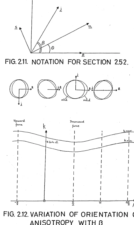
Wavenumber, frequency relationships Anisotropy ratio-frequency dependence Phase-velocity, wavenumber relationship Notation for Section 2.5.2.

Variation of orientation of anisotropy with~

To illustrate the resolving effect of,the wave on j and B

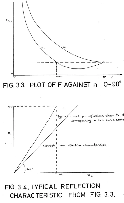
Reflection construction - anisotropic waves Reflection construction - isotropic waves Reflection function F v n, 0 - 90°

I

.

:

3.4

Typical reflection characteristic, from fig.

3.3.

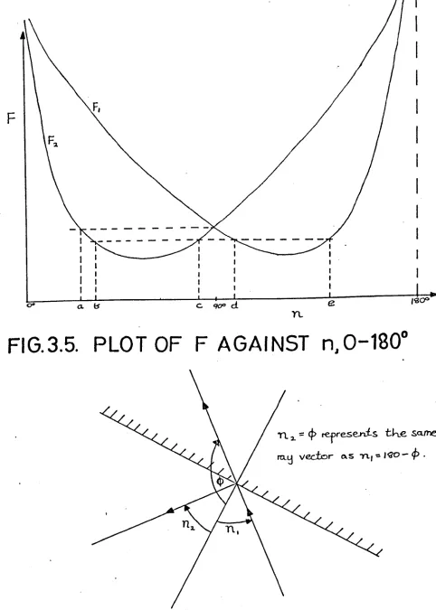
3.5

F

v n,

0 - 180°

3.6

To illustrate the meaning of n

>

90°

3.7

Notation for analytical solution of reflection problem

3.8

Computed reflection characteristics

3.9

Wave reflection pattern when r

>

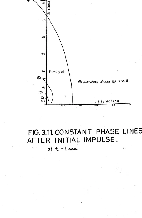
90°

3.10 Wave pattern after initial disturbance - ignoring surface tension 3.11 Computed constant phase lines after initial disturbance - mercury

3.12

Detail of fig.

3.11

(c)

(vi)

3.14

Notation for refradtion problem

3.15

3.16

3.17

3.18

3.19

'.3.

20

3.21

3.22

4.5

4.6

4.7

4.8

4.9

4.10

4.11

4.12

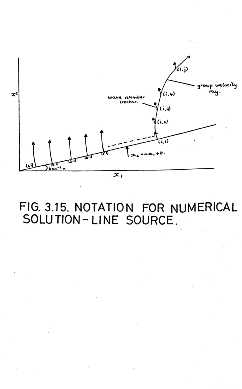
Notation of numerical solution, line source

Computed plots of group rays, line source, linear variation of ~

Computed plots of group rays, line source, quadratic v~iation of

'If .

Computed plots of group rays, point source

Lamb's typical ship wave pattern Notation for Lamb's method

Notation for Ursell's method

To illustrate method of plotting lines of constant pbase

.

°

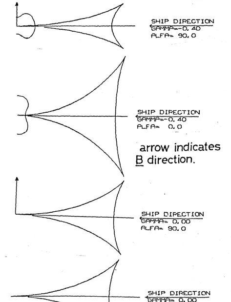
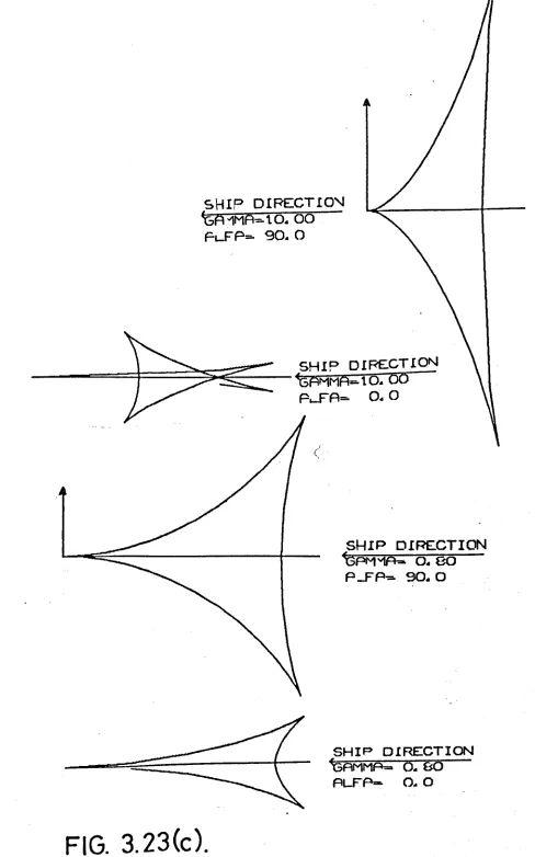
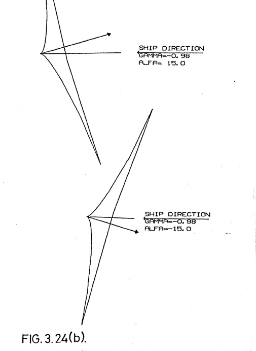
Typical H.H.D. anisotropic ship ...rave patterns,o<.= 0, 90

0' 0

Typical. M.R.D. anisotropic ship wave patternst~=

.-15

,

.+

15

'1

30°, 45°, 60°, 75°,

Total anisotropic ship-wave pattern to be expected. Computed wave crest patterns for the fish-line problem

Photograph - Tank for mercury experiments

Photograph - General view of equipment for mercury experiments Optical path for wave observation in mercury experiments

Photograph - Typical wave pattern observed in mercury experiments Photograph - General view of ancillary equipment

Photograph - Vie\V"of Relmhol tz Coil magnet Magnet conductor section

Photograph - Flow monitor

Magnet protection electrical circuits Magnet calibration curve

Axial field plot Transverse field plot

4.15

4.16

4.17

4.18

4.19

4.24-4.25

4.26

4.27

4.28

5.5

5.6

5.7

5.8

5.9

5.10

6.1

6.2

(vii)

Sketch of details of large tank Photograph - Large tank in position Photograph - Smaller tank

Photograph - Overall view of equipment Photograph - Plungers used to produce waves Expected flow produced by disturbed surface

Photographs - Anisotropic waves from a point source Photographs - Waves from a line source

Anisotropy ratio plotted against the parameterA~

ufg

Photographs - Waves from a line source, different ~rientations Wavelength ratio plotted against orientation

Sketch of false floor for wave refraction experiment Photographs - v/ave refraction

Photograph -'attempted wave reflection

General notation for m.h.d. Rayleigh Taylor problem

The effect of inclined ~ upon surface inclination, notation Variation of surface inclination with magnetic field inclination Plane of instability when heavier fluid is lifted above lighter fluid by j x ~ force

Comparison of menisci for different j

x ~

forces Comparison of menisci for different liquids

'2)'

Typical tank configuration for

~~;6

0

~'

Predicted surface profile for ~~

=F

0

Mathieu function stability diagram

jB to produce instability for a given ~

min

r

(viii)

6.3

Photograph - depth probes 6.4 Circuit for resistance probes

6.5

Typical calibration curve for resistance probe

6.6

Circuit for T-probe

6.7

Photographs - Effect of Teepol on meniscus

6.8

Surface profiles plotted using resistance probe

6.9

Photograph -

i~

=/:::. 0 instability in large tank

6.10 Photographs - Sequence to show 'bridge' instability

6.11 Photographs - Interfacial instability when

~=F-o

6.12 Photographs - Effect of magnetic field alone on .fluids of different

J1

6.13

Photographs - Typical photographs from orientation experiment 6.14 Plotted results of orientation experiment.

TABLES

(ix)

NOMENCLATURE

Other symbols used occas\,ionally will be defined as used •.

-li

I1agnetic field strength

c Phase velocity of waves

C

Group velocity of waves g acceleration due to gravity

h depth of fluid

i unit vector in the vertically upwards direction points

Variables definingl in the Electric current density

numerical solutions of

"

k,!f_ vlavenumber,wavenumber vec tor

)11-)1,

--_;;..__- a type of dynamical viscosity term

f-a.-f1

Instability time constant or frequency (chapter

5)

M

n

n Co-ordinate "axis normal to a given surface

p Pressure in fluid

p

p

Point in a numerical solution Stress (normal and shear)

s Co-ordinate axis lying along a given surface

t

Time

u,U Speed of travelling disturbance Fluid velocity

x

Dummy variable in computations for shallow fluids

x,y

Horizontal co-ordin~te axes

z Vertical co-ordinate axis

Surface tension

Angle between 'mirror' and ~ direction in

§

3.2

Angle

between 'ship' direction and

&

in

j

3.5

(x)

j5

Angle between j and ~ if not assumed as 90°

j)

Angle used in ship wave solution, for

§

3.5.2 see fig(3.20),

for

§

3.5.3 and 3.5.5. see fig(3.21)

E

The difference in the value of a parameter across an interface. Dirac's delta function

A small quantity

Surface or interface level Angle between

k

and ~

e

Angle ~ makes with horizontal in

S

5.2.2

A

Wavelength 1

Viscosity

Hagnetic Permeability in

S

5.3.4

-,

Kinematic viscosity

jA1

+jJ..t

-- - a type of kinematic viscosity term

p,

+

f1

-Density of fluid

i:

Summation symbol

a

Frequency

CJ Fluid conductivity in

S

5.2.4

Velocity potential in the wave solution Phase function (chapter 3)

Surface angle to the

-1 Ca

tan -- in

Ck

horizontal in

"

Part of velocity 'potential' term in viscous waves solution Vorticity

(xi)

Subscripts

:-i,j denote co-ordinate directions in vector differential expressions k denotes wavenumber direction

n denotes normal to wave crest (ch 2) n denotes normal to surface (ch

5)

p,q denote directions parallel and normal to the 'mirror' respectively in

S

3.2

s denotes along wave crest (ch 2) s denotes in plane of surface (ch

5)

0( denotes all relevant co-ordinate directions in 'summation

terms

e

o

1

2

1

2

normal to wavenumber direction "

indicates value of parameter at surface or interface denotes j direction in

§

3.4

denotes B direction in

S

3.4

(xii)

ACKNOIVLEDGEHENTS

I wish to express my thanks to all those who have contributed to the development of the work described here, and towards the production of the thesis itself.

In particular I must thank P~ofessor J.A. Shercliff, my supervisor, who first suggested the subject of H.H.D. anisotropic surface waves as a topic for research, and who has guided and encouraged me throughout. Thanks are also due to Dr. C.J. Alty for help with practical arrangements in the

laboratory.-J-;r.P. Worsnop of U .K.A.E.A., Culham, supervised the -, design and construction of the Helmholtz Coils described in

Chapter

4.

Various members of the workshop staff in the Warwick

until success was achieved. The cheerful assistance of Mr. Colin Major University engineering department helped to build the equipment

described in the thesis. HO\...ever, in this respect I pwe the biggest debt of gratitude to Hr. Alf. Webb who not only helped to make the equipment work smoothly through his skill and effort but also encouraged me to persevere with the experimental work _

in developing the equipment, and of Nr. Alec Ross must also be acknowledged.

I thank Hr. Colin Lovatt for help in processing the photographic records of wave patterns. Tharu{s must also go to Miss E. Peatman who willingly ruld patiently typed this thesis.

The work was carried out whilst I \...as on a research studentship from the Science Research Council, whom I thank for

i'

_,

financial support.

Finally, I want to thank my wife, who helped in drawing diagrams and other editorial work on the thesis, for her patient encouragement and support throughout all this work.

1. INTRODUCTION

1.1.!he

Neture and Scope of the Research

Problems in magnetohydrodynamics

(M.ll.D.)

can be loosely

ditided into three types;

those of kinematic H.ll.D. where the'

motion of a conducting fluid which influences the electromagnetic

~ameters

is giTen ab initio,and

essentially the solution is

merely an exercise in electromagnetic

field theory;

those where

the problem is basically one of fluid mechanics, with the Lorentz'

(j

x ~ )

force, imposed and invariant from the start, acting as

one more (albeit possibly rotational) force acting on the fluid

along with pressure gradients, gravity etc.;

and those w~ch

exhibit a true 11.H.D. coupling where the fluid mechanical and

electromagnetic

equations are interrelated and cannot be solTed

independently.

The research presented

in

this thesis is

basically to do with problems of the second type, although in

fact the phenomena described could not occur were it not for

a particular mechanism whereby the fluid mechanical parameters

feed back to influence the electromagnetic

ones.

The subject is the study of the waves, instability,

and the stationary profile of the surface, or interface with

.an insulating liquid, of a conducting fluid which is subject

to an imposed magnetic field and carries an imposed electric

current, such that the resultant

j

x ~ force is irrotational.

To the extent that current and field are both imposed, the

•.'

problem is of the second category, but the particular coupling

effect 'referred to above is that the current always tends to

"fill" the conducting fluid, and so at the surface of the

fluid-it is always to be found parallel to the surface.

" "

2

-In this way the fluid motion, or more strictly the motion of the liquid surface, is able to influence the electromagnetic

forces, and the result is strong anisotropy in the wave dispersion and instabilities.

The basic phenomenon of anisotropy 1n the above circumstances has already been reported by Shercliff

(1969)

in the case of waves, and in instabilities by Lemaire

(1963)

and others. The original theoretical work in this thesis has been to examine some of the implications which this anisotropy has beyond the simplest cases already solved •.

"

Thus a number of classical surface wave phenomena have been

applied to the case of anisotropic surface waves, with interesting results. In the stability problem an attempt hqs been made to study the effect of small variations in the configuration of electromagnetic parameters upon the instability motions, with the result that novel instability modes have been discovered.

The experimental work has been to demonstrate the

anisotropy, which has not been done before, to show its' influence on other wave phenomena, and to discover what effect it has on various configurations of instability.

'.2.

The Evolution of the Research

The whole of the work reported here grew out of an initial attempt to demonstrate experimentally the existence of anisotropic surface waves. It soon became apparent that further theoretical work needed to be done to predict accurately the practical

3

-Most of the work has as its goal the academic aim to

inquire, learn and verify;

it is not related very closely to

current technological needs, but since M.H.D. is a relative-ly.

new, and still largely uncharted subject, it was thought well

worthwhile to explore this corner of it relating to free surfaces

and interfaces under imposed

j

x B

forces.

As far as is known,

the phenomena under investigation do not occur naturally in the

universe.

In

the instability work

in

particular, although the

results are presented in a lo~ical sequence, it would be f~se

to pretend that the particular problems dealt with \"ere

in

practice posed, solved, and experimentally verified, in that

order.

Rather, only when the instability mechanisms were

better understood through a combination of theoretical study

and experimental work, 'and the answers effectively obtained,

could the questions be posed

in

the '"ay set out

in

chapter

5.

Thus the overall philosophy with which the research was approached

was one of going step by ste~, asking questions and finding

answers as the understanding grew, rather than starting with

the research mapped out from the beginning.

The interplay

between experimental and theoretical work has fostered this

approach, which is somewhat unusual in

t-l.H.D.,

a subject

in

which

it is not often easy to match experimental and theoretical progress

and let each influence the other.

One practical aim which does lie behind the wave experiments,

"

although not developed as yet, is that of using the anisotropic

4

-for the general study of anisotropic waves

in

physics.

It was

this Rim which prompted the theoretical study of the application

of the anisotropic

dispersion relation to classical surface wave

problems, since these could be the very things used to visually

.demonstrate

the sometimes unexpected

properties of anisotropic

waves.

Finally, it is worth recording

that a ten month delay

in

the delivery of the central piece of equipment, the large Helmholtz

coil magnet system, has seriously limited the progress

in

experimentally

demonstrating

all the wave phenomena it was hoped to show.

Layout of Thesis

"

The thesis is in two broad sections, chapters 2, ,and

4

on

anisotropic

surface waves, and chapters

5

and

6

on the M.H.D.

Rayleigh-Taylor

inl3t~hility and related

pr-obl.ema,

Ch"lpter 2 is

':l

deb-dlc,.lstudy

('If

the basd,c anisotropic

wave problem,

RS

a preliminary to the experiments,

and so contains

Borne of the work alre,9.dydone

by

Shercliff,

as a basis, but the

rest is original, computing and plotting theoretical dispersions

involving surface tension, the solution involving viscosity, and

discussion on the nature of the anisotropy.

Chapter , moves on to deal in more general terms with the

application

of the anisotropic dispersion to classical wave problems,

and is more

en

exercise in kinematic wave theory than M.H.D.

There is a review of methods of wave kinematics

developed by others,

and then these methods are applied successively

to

(a) the reflection

of anisotropic

surface waves,

5

-i.e. the pattern of waves to be f01md a given time after an instantaneous point impulse or point surface displacement, (c) the refraction of waves due to j varying in a plane normal to

,!!,

and

(d) the problem of finding the pattern of waves when a disturbance moves steadily across the surface - the "ship wave" problem, or when account is taken of surface tension, the "fish line" problem.'

Chapter

4

describes the experimental work to demonstrate the existence of anisotropic surface WllVes, and to show soma of the phenomena of chapter

3.

This covers 'the consideration of possible experimental approaches and choice of suitable parameters, the design and operation of equipment, and the results obtained.

Chapter

5

covers the theoretical aspects of the work on th~ Rayleigh-Taylor instability, with a section on the effect ofj x

,!!

forces on the shape of stable liquid surfaces, a brief resum& of the simple H.ll.D. instability case already solved, and then investigation into the effect on the instability of varying

j and ~ whilst still maintaining irrotationality.

In chapter

6,

the experimental work on instabilities is detailed, including a description of the equipment, the development of surface-height sensing probes, and a novel large-amplitude

instability which was discovered, as well as attempting to verify the phenomena predicted in chapter

5.

Finally, brief conclusions are drawn in chapter

7,

along with suggestions for further work.

Where possible figures are bound next to the relevant pages of script. Some information, not considered relevant to the main text, is relegated to the appendices, notably specification of '.

6

-which are simply copied out.

Since the programmes were

merely used as tools to solve lengthy equations, both directly

and numerically,

and to plot out results, no attempt has ~een made

to describe their operation except the numerical plotting of

group rays in chapter

3,

since computing at this level cannot be

considered an end

in

itself, but merely a means of solving

problems it would be otherwise time consuming to solve by hand.

",

-w"

7

-2.

ANISOTROPIC SURFACE WAVES UNDER A VERTICAL

j

x

B FORCE

2.1.

Introduction to the Problem

2.1.1.

Outline of chapter contents

In this chapter, the basic theory of anisotropic surface

waves

in

a conducting liquid is examined.

When a horizontal

.

magnetic field and horizontal electric current are imposed on an

electrically conducting liquid, producing a vertical electromagnetic

force, waves on the surface of the fluid, which must be excited by

external means, propagate at different speeds in different directions.

The foundation of this theory is the work of Shercliff

(1969),

the

salient features of which are outlined for completeness

in'

2.2~ .•..

".

since they form the basis of the rest of the original work relating

to the anisotropic surface waves'.

In 2.3 the analysis has been extended to cope more

realistically with experimental conditions.

Theoretical predictions,

.

are obtained from a dispersion relation for waves at the interface

between two liquids, with surface tension taken fully into account

and an attempt has been made to analyse the effect of.viscosity

in

both liquids.

In 2.4 the computational solution is described and polar

plots of phase and group velocity and lines of constant phase ~e

presented, along with a discussion of their implications.

In 2.5 the fundamental nature of the anisotropic effect 1s

discussed, in an attempt to isolate the true M.H.D. aspect of the

phenomenon.

Finally, the effect is considered of varying the angle

between the imposed magnetic field and electric current directions, .

for the practically possible case involving surface tension.

,c

The aim of the work

in

this Chapter has been to take

the-theoretical base of Shercliff, and modify and present it

in

a form

· 8

-2.1.2. B~sic assumptions and approximations made

These are the same as those made in Shereliff

(1969).

Small amplitude waves are considered in every cl'l.seso that only the linear terms of the hydrodynamic perturbation equations are necessary.

,

The magnetic field is imposed horizontally and is supposed I steady and uniform throughout and the electric current due to an applied D.C. electric field is assumed to be horizontal and of uniform density throughout the conducting fluid in the undisturbed ..state. Thus the liquid surface is normally at rest horizontally

under gravity and vertical irrotational j x D forces.

The magnetic induction due to the imposed curr~nts is assumed negligible compared with the applied field, and induced currents due to wave motion in the presence of the magnetic field are also neglected. These assumptions will be justified later in

chapter

4.

In general when the surface is disturbed vertically the distortion of the current density field will give rise to rotational

j x

.!!

forces but we shall assume the waves to be of small enough amplitude for this to be ignored.

2.2. Previous lvork

2.2.1.

General Literature

Helcher (1963) gives a fairly comprehensive description of field coupled H.H.D. surf~ce waves \'Ihichin some cases are anisotropic but those are a different phenomenon from the one under consideration here, being. for cases where the electric and magnetic fields are not effectively independent, and are an integral part of the wave

propagating mechanism.

9

-2.2.2.

The basic dispersion relation

(Shercliff.

1969)

Using the notation of Fig. 2.1. we consider a plane wave

train of frequency rowith normal

in

the n direction, trougns and

crests in the s direction.

js' the component of imposed current in the

s direction will not be perturbed by the waves whereas

j

is perturbed

n

in the z,n ~lane,. and

in

fact in this plane, the current at the surface

follows the surface profile.

Thus it follows that curl

(1

x ~),

( =

(~.grad)

1

since div

1

=

0 and ~ is uniform) has zero

8

component.

Now the linearized perturbation equation of motion

is:-()" J .

B

.

f

d~

+ ~

f

=

j_x_ -

r'3 ~

• ••• 2.1 .

neglecting viscosity, with all variables harmonic functions, of timd

h

is a unit vector in the

+

z direction.

Taking the curl of (2.1) gives

which has no s component, and so

=

0 which requires w

=

0 if

1,\

is a harmonic function of time.

-s ='s

Therefore it is possible to define a velocity potential

~ (z,n,t) for the irrotational flow in the z,n plane.

Now

lx

B in (2.1) may be expressed as

-j

B

i+ j'

x

B

+

j'

x

B

s n- - -8 - -n

where.it is the current vector in the z,n plane.

j

t x B

acting

n

J:iorizontallympy be neglected as small in this small amplitude

approximation,

whilst it should be noted that

j'

x B

will be

iri

the

- -s

z,n plane, and at the surface will always be normal to the surface.

Thus (2.1) may be expressed as

:-()9>

g_rad

(P

~t

+

P

+

(f~

+

JsBn)2)=

l'

x

Bs

••••2.2

If this is integrated along the surface z

=

z ,

j'

x B

o - -B

contributes nothing, and if the ambient pressure above the surface

j

I e.

j ~

+

jn.

1

-

-

-'Z

" JT\.

1

L

(U"Lt ve.c.tor)

-

10-with

. I

and hence all the variables

are harmonic functions of n.

":I.

~ Za

k1.

For surface tension

c:J... ,

at the surface, p

=

-ex. ~

7\.\, = ol.Zo

to a first approximatiOn.

Hence, at z

=

0

(applying the classic linearization

process such;

that all variables are the same at z

=

0

as at z

=

z

)

o

'.

••••2.3

(2.3)

is effectively the boundary condition on pressure

at

the

surface.

.

The motion of the fluid as a whole is defined also by the

two-dimensional

Laplacian

\7

'1.

¢

=

0 ,

•••• 2~4.

since we assume incompressibility,

and

by the boundary

conditions:-_ ~ _ ~"Zo

V.,_ -

~z. -

~

~

"dz.

at

z

=

0

' •••• 2~.5

and

= 0

at z

= -

h

•••• 2.6.

in a bounded fluid of depth h.

(2.4), (2.5)

and

(2.6)

require a

form:-cf

=

C

r

9

e,

,(Cot -

kfl)

f

sink

k

2.

HOt.)..

kit

"",.,I..

b] ...

;2.1

'For

(2.3)

also to be satisfied, a constraint relating ~ and k

is required, and this is the dispersion relation.

Substituting

(2.7) in (2.3) gives

:-1

(k~o(.""

f~

+

js

B,,)

•••

2.8

N.B. A somewhat different approach to solVing for the dispersion

relation may be found in chapter

5

where the stability equation is

effectively the same as the dispersion relation.

Thus it can be clearly seen that of the field and current

components, only js and Bn affect the dispersion relation.

This'"

11

-produces anisotropy of wave propagation, since the magnitude of

"

j B

varies with the orientation of the wave number direction

Ie ,

s

n

relative to the imposed

j

and B fields, and given that oo-is fixed

there is directional variation of

I~I

2.2.

3.;

Predicted results

Shercliff went on to eValuate the sort of results to be

expected from the dispersion relation

(2.8)

in both the case of

"surface" waves on a deep fluid, where the wavelength is short

compared with the depth;

and "long" waves in shallow fluid,where

the depth is small compared with the wavelength, and vertical

accelerations

can be ignored; i.e. tanh kh

=

1, and tanh kh

=

k h

'.

respectively.

oB

Taking

i

=Las

a

dimensionless parameter indicating the

f3

relative strengths of J_x

B

and gravity forces, and,ignoring

surface tension to simplify the calculations;

and considering

the case where

j

and B are imposed mutually at right angles, to

-

-

,

produce

1-

x

.!!.

upwards, equ.

(2.8)

reduces

to:-=gk

(I -)'

Cc":)'1.

e )

for surface waves and

••• 2.9a

2

00

for long waves,

•••

2.91>

where

e

is the angle between the

k.

and ~ directions.

This configuration of imposed fields produces the greatest

degree of anisotropy, although there is

a

stability limit of

)5<

1

if the net force on the fluid is not to be upwards, causing the

,

Rayleigh-Taylor

instability to occur.

Shercliff presented the anisotropy visually

in

polar plots

of phase and group velocity,

(see

2.4.1.

and

3.1.3.)

and these are

shown

in

fig.

(2.2),

adjusted to suit the particular case of the

1

1. d.i.rec.ti.,."

(i)

Pha.se Ve.lo~i.t~

r

a)surface waves

a

I

i

ti)

Ph.a.se.

V L

_.

t

_-

j tlirf".ctio",-

...

e

OCL ~

. 1"1

V L

.

t

J cl~,.!:C-t';ot\,

OJ)

G

rou~

e

OCL. ~. ..

b)long waves

.FIG.2.2.

SHERCLIFF'S'

DISPERSION PLOTS

12

-is drawn, and the complete picture -is obtained by reflection in

both axes.

The salient features to note as characteristic of the

dispersion are that waves propagating in the

j

direction are

unaffected

by the

j

x ~ force, whilst those in the

B

direction are

most affected, to the degree that when

~= +1

the waves will not

" ,

propagate at all.

For wave~ in ;-ther directions ,-the eff;ct is

somewhere between the two extremes, and of great interest is the

fact that the phase and group velocity are not in the same direction.

Lines of constant phase due to a continuously oscillating

point source, i.e. the trough and crest pattern which would be

observed in an experimental situation, are identical in shape to

the polar plot of group velocity for the dispersion relati~n6

specified by eq. (2.9).

~

"

"

2.3

AdaptAtion of Theory for Practical Situation

2.3.1.

Waves at a two fluid interface

Now the first'aim of this project was to demonstrate

experimentally

that the anisotropy of B.Il.D. surface waves exists

.,

at all, and to do this I had to determine how to show up the.

anisotropy

to best advantage.

From some of the practical

considerations

to be found

in

chapter

4,

it became clear that

"

probably the best way to obtain suitablp. waves was at the interface

between two liquids of very simil~r densi.ties, one electrically

. conducting,

the other not.

Usin::;tl:ese, t~1.e

gravity force

influencing the waves could be reduced by an order of magnitude,

making it practically !,>ossiblefor the

j

x ~ force to "compete"

with the gravity force.

In this case, the dispersion relation is obtained assuming

the anisotropic effect of

j

x B as discussed above, simply adding

-

-2

the

j

B cos

e

term where appropriate to Lamb's analysis

(Lamb 1932 Art. 2.31 ) and it is supposed therefore that iand

B

·fN·f).Tht, ,..~

~~

,-L:,~~ ~ ~

,9.

i..?'

~l

~

~

~

U1.. ~

~

~

w-k ~~

t.~ ~~

e'Otk ~

~

..a ~~

13

-are applied mutually at right angles and that j x B acts upwards,

-

-

.

and

e

is then the angle between the wave direction and the magnetic field.

If subscript (1) denotes the upper non conducting fluid, and (2) denotes the lower conducting fluid, the analysis is as '

follows.-In the upper fluid,

V\1>,

=

0 In the lower fluid, \7~<P~=0

)

)

)

the wave number vector ••• 2.10 In a vertical plano containing

t

being a two dimensional velocity potential, as we saw in Shercliff's analysis.

The equation of motion

is:-grad

(f1~+:P'

+ f'1~Z_)

=

0

grad

(P:z.~+l''I.+[F2.~-~BOo'lSJ2..)

= /

x ~s

At the interface,

1.

x ~ is always normal, 60 integrat?-ng

~ ~, •••: 2.11a

•••

2.11b .

(2.11b) along the interface z

=

p,..<

;P

t""

)z.Zo

.

+.plo

+

(P2

g

and (2.11a) gwes

fl( ~~\"ZO

z

gives:-o

2

- jB cos

e)

z

=

0

o

+:p,

+

p,

g z0 = 0

•••

2.12

•••

2.13 Now the interfacial condition on pressure at z

=

0

is:-b~Zo

r

2.

=

PI -

0<. ~ 'l'\.z. • •••

2.14.-••• from (2.12), (2.13) and (2.14)

Jt

••• 2.16

But

Now if the interface

_•••

2.17

(2.10) can be solved using (2.16)

~

boundary conditions ~z

=

0 at z = + hl and

~d (2.17), with the

"?J¢,_

-= 0 at z

=

-h

d2. _2

14

-LW£.

t(wt-kon)f

k

k

]

Thus ~,

=

k.e.

- -

s~

2. - coth.

h,

co,!;

h.

b~ol

rl, \.w

£.

i

(w

t: - k0

t\)f

I

k

]

'"1''1.

=

T ~

--

[SiTU\. "2.

+c.oth

khl..

C6Sh.

boa.

r

0 •• 2.18

For (2.18) to be compatible with the boundary condition on pressure, (2.15), the constraint necessary is the dispersion relation ro

=

f(k)

obtained by substituting (2.18) in (2.15) and

(

~

)

assuming that

"dt 2.a-z.o

Hence:-••• 2.19

From this it can be seen that the two fluid case is essentially the same as that of the surface waves on a single fluid in contact with vacuum or gas, since had we introduced,

j x B acting downwards in the upper field, l-l1ththe lower fluid

-

-non-conducting, the dispersion relation would have been identical (showing that the anisotropy term j B cos2

e

is independent of the actual fluid parameters used).

The final choice of experimental parameters is discussed in chapter

4,

but it is worth noting here that the degree of anisotropy obtainable will depend upon the right hand side of (2.19),

in°

». particular the ratio

t-Oompardng rthd.ewith the single fluid case it can be seen that if

(f'l..-f1)

is made very small, j B can compete with it all the more easily, though of course j B must not exceed

(f'l. -

f1

)g or else the Rayleigh-Taylor instability occurs. Whereas in the single fl~id case negative j B (i.e. downward acting j x B )

15

-upward force, here, if

(P1-

f1)g

is an order of magnitude less than

j Bt as is possible by almost equalising the two densities, then a large degree of anisotropy is obtainable with a downward j x B too,

-

-with no problem of inst"1.bility. Cert~inly the possibility of varying the ffi3.C;nitude of the term

(f'2.. - (',)

offers more scope for obt<:>inin:!suitqble ex:,erimcntal parnmet ez-s,

2.3.2. The effect of surface tension

Shercliff, to show up the b".sic phenomenon to best advantage, and for ease of manipulation chose to ignore surface tension effects in plottin5 the sort of shapes of wave pattern to be expected

(fig. 2.2). Whilst this is justified for that reason, ;t is misleading when approaching the problem of actually generating such shapes in practice. One might initially assume that given a large enough space. dimension, waves of sufficiently long wave-lengths could be produced for surface tension effects to be of no practical significance. However in the extreme cases of anisotropy the theory predicts zero or nearly zero wavelength in the directions where the j x B force has most effect. So that however long the usual wavelength of the system is, there would always be present some wavelength short enough to be affected by surface tension. However- small surface tension is, the more severe anisotropv could not be achieved in practice for this reason.

2

Looking at eq. (2.19), it is the size of the dlk term

2

compared with (

('2.. -

f1

)g - jB cos

a

which determines the extent to which surface tension is important, but of course k itself ie the dependent variable in this equation for most situations

16

-possible

to determine the overall effect which surface tension

does have on the pattern by simply introducing

some sort of

correctine

factor.

In fact it is true to say that here-is

a fluid mechnnics problem where the exclusion of surface tension from

the analysis has a qualitative as well as quantitative effect.

Thus

eq.

(2~19)

must be solved as it stands, and this is done

in

2~4.

2.3.3.

The effect of Viscosity

Since

in

the search for suitable experimental liquids

a number of otherwise possibly useful ones had a viscosity an

order of magnitude higher than water, which is usually ~on61dered

inviscid

for surface wave propagation problems, it was thought

necessary

to determine by analysis what effect, if any, viscosity

has on the anisotropy.

Moreover,

in the two-fluid case, the

wavelength

for a given frequency is less than for the free-surface'

case, and it is not immediately

obvious whether this would result

in

more or less damping of energy by viscosity, whilst there is also the

effect of shear stresses at the interface to be taken into account.

As far as coUld be determined,

the problem of solving the

'

";

wave equation, with viscous effects, for the interface between two

liquids, has not been tackled

in

the literature and so it is set'out

below, using Lamb's analysis for the free surface case as a guide'

(Lamb

1932 ~ 349).

The axis notation is es shown in fig. 2.1, subscript 1 for

upper parameters

and variables, 2 for lower.

The equations of motion

in

the z, n plane

are:-•••

2.2Oa

17

-and diVe !!1

=

dive !!2

=

0

••• 2.21

where the vectors are two dimensional with

z,

n components.

(2.20) and (2.21) are satisfied by

d

q,o(

'd

Yo(.

a

<Po*. ~

YoI,

r.

Uo(.'l1.

= -~

-

~£.. '

U",2.

=: - ~'Z.

+

d1"\.

Lex.=

1, 2J

•••

2.22.

with

V\p

=

0,

t~

~

\J"2twhere

Vl.

is a two dimensional Laplacian operator,

_•••

2.23

with

'P1

=

..:..:a. -

del>

gz

P1

dt

1>'1 ~~2.

(g

+

jB

cos2

e)z

-=

--f'-

~t

_f2.

•••

and

_•••

ikon.

+

crt

On assuming the variables to vary as

.e..

the solutions of (2.23) are

:-CA

-b,,"

B

1<:20)

1

e

+ 1 ~

~=

ik'l'\. +

crt

.e:

ok

t}

Z>O

l n

+0-e.

cf>'l.

=

(A ~

'f,_ -

(C,-••• 2.25

where

'2.

I'l.

0-ltJ1o( -

<

+-Voc.

•••

2.26

It

the fluids hsve infinite height And depth (for simplicit

y)

+

then one boundary condition is for zero motion at z

= -~

Hence B1

=

B2

=

0, and providedtn~has

its real part positive,

18

-Substituting

(2.25) in (2.22) gives

( \ R

-kz.

C

-~I-z..)

t:b".u ....

t:

)

U.

?It

-

- l< 1e.

- m,

1e,

e.

₎

+

(kA

1

e--

k-z.

I

-",,4)

u«

nof- tr i:

)

LlZ.1 of-

i

<.

e,

-e, e,

)

)

( kz.

M"2.)

ik'J'\.-ttt-l

)

•••

2.27"

Uh1

-

_l

k

R

_{'J. -e, t-}

_m:z.

_{(2-e ~}

e

)

~

(I

k2

'kC

m~"2.)

i.k-~.,.o-t:

UZ1

_-

_<..

_A'J..e.

_-

_{L 1}

_.e.

_.e:

₎

)

If

z =

'l.

denote the inter'fa.ce,with ~

= 0

the undisturbed level,

~

then

~t

=

u

z1

=

u

z2

at the interface, is ~other

boundary condition,

and the small amplitude a~proximation is made that

d!l -

(l! "\

-

(u )

)t - 21 )2.::(!) - Z2.. 2=0

"

k .

)

'I

t:

k

)

lk'Y\+o··t

- (R

..

C

L {')I.·flr - -_

(R

-lC

..e

Hence

1.,::::-

er

f t L t

-e.

-

er

"l.:z. •••

2.28

The other boundary conditions are those due to norma.l and shear

stresses,

viz : -

P'l..2.'1.

-

P1Zl.. = 0<..

;'l~

and

,

where

0<.

is surface tension

_•••

,

2.29

But

_•••

Substituting

for

pvC.

from

(2.24)

at z

=

1t,

with

fat

z

=

0

(

)

d

Ut\~ ~ U·UI. ~u2.OC

from

2.25,

and substituting

for

d"Z..

,~'

~

from

(2.27)

gives

R2:Z. /

Pt

=

f_-o-+-~

-2.

v,

kl.] At

+ [~ ~ -

2.

111

km,,]

L

(1

I;1tjp&

=[-o--(~+lB~l.e)~

-2v~k

J

A~+[(3+SB~:Le)~t2~k~1] ~

c,

ft1\.'Z.

==)L,

[2

i

k't

A1 -

(k'4t'W\11.)

e,

J

.

D ••.•

2.31

rl.'M.

==

)1'l.[-1Lk1A:),-(k2t1n1~)C2]

(2.31) in .(2.29) gives, with

j

B

Co?

z

8

=

r ,

A1

=-li";l

,C,=

C2.

t~om

(2.28)

[ (f'-

+

(>1)

0-

+ [ (

f:t -

Pi) ~

+

r] ~

+

(y,_

+!-1)

2 k~

+ ~"

3]

A

1.

19

-••• 2.'3

Combining

(2.3~)

amd

(2.33)

to eliminate A1 and C1 we have

(f'.

+

(1)O-(f'.-J')2

k'

+

0'':_J',~4-

k~

-+-

(r:-(',')",' .,_

(re

('.)\k

~(f.-

('0

rk

+~> -

f,)(?'

+

f,)2

k

'a-

+ '"

k'(P'-('1)

=

4-

k?

(fl."'"

+jL.

'lny{P.j!~

and

_{frequency without viscosity}

for the given wave number k)

•••

2.34

This is the dispersion relation.

The simplest case is.when

jA,

c

r- ,

Then

cl

+

w2

+

)J1'1

:.1

k

'l ~

=

0

• •• C1

= -

k'l)}11

±

J

k~

V,.,,'). -

(.U l.

M=O

•••

This case gives at least an approximate guide·to·the

Bort of beh~viour to be expected

in

the more general case.

For the present, what matters is the extent to which the viscosity

alters the wavelength for a given frequency, as this would alter

the anisotropy, and also the magnitude of the wave damping.

·Both

k~\

I

effects depend upon the size of the term

vM

The former effect·is negligible for

w2

»

k

4

)JMl.

Whence

a c -

k2){,

+L

CV , since the

term

iw,

which contains the

anisotropy, dominates the magnitude of

C1.

The effect of having two fluids is to increase k for

20

-the viscous term, which effectively sets a limit on the closeness to which the liquid densities may usefully be matched. _Similarly,

in the case of an upward force

(r

-ve), the usefulness of increasing the magnitude of

r

is limited, si.ncek is thereby increased in one direction, increasing the influence of viscosity in that direction. However, with a downward force, if the frequency is unaffected

by

viscosity in the o.h.d. case it will be unaffected in the

M.H.D.

case. For

en

upward force, it is worth noting that the viscous term will increase as the square of the anisotropy ratio between

k~

l.

smallest and largest wave numbers encountered, so that

)}M

could possibly increase by two orders of magnitude. This' suggests that viscosity may not be negligible even ,...ith the use of fluids such as water normally considered inviscid for wave propagation purposes, and certainly discourages the use of more viscous liquids. The limiting effects of viscosity on the size of frequency and wave· length to be used in practical cases will be considered in chapter

4.

I" The general interpretation and solution of eq. (2.34) is more complex, since after substitution for m, a polynomial

ot

order 8 in

a

is encountered. It is interesting to note that the consideration of two fluids has the effect, via the right hand side

of

(2.34)

of doubling the order of the equation. In practice,

some of the terms may well be negligible compared with others, and in chapter

4.

the equatirm will be examined with pertinent v'llues inserted.

Thus although (2 •.311-)does not re~dily give a cle'l.ridea of what happens when viscosity dominates, (i,.e. when the problem is no longer a true wave motion. problem, n!J.vingodd order terms in (J comparable in m~gnitude to even order terms), it does enable

ih~

21

-results of an inviscid solution to be tested as to the validity of the inviscid assumption.

2.4

Theoretical Predictions

2.4.1.

Note about phase and grou!' velocity and lines of constant phase

Since we are dealing with anisotropic waves, dispersive with respect to direction as well as frequency, distinction must be made between polar plots of phase and group velocity and lines of constant phase (at unit time after that phase has left a point source),

whereas in an isotropic system all would give polar plots that were circles, although possibly of different size. The dispersion relation so far has been expressed in the polar

k

plane, ~.e.

ro

=

f(k,a) where k is the wave number of wave crests lying normal to the

e

direction. In this situation the phase _{velocity c}

=

.ttj

k, '

, .

The group velocity, the speed of wave cr-eabs , is in the

e

direction.

which may be thought of as the speed and direction of a packet· of waves with a given k and ro or equivalently as the speed of propagation of energy contained in a given ro,

k

mode, has components

It.both ptlI'alleland perpendicular to

e.

1

(~UJ.'\

and

Co

=

k

'deA,

c and C(

=JC:+C:)

are conveniently displayed in polar plots • These are C . c

le

for a given

~w

(~)e

:- Shercliff

(1970).

22

-relation includincr surface tension, k~ F(e)

G(w)

so that, referring to Shercliff

(1970),

the lines of constant phase are not the S3me shape as the polar plot of group velocity. This is because the vector representing the constant phase curve bears a ratio to the group velocity vector which varies with the wave number dire~tion. The line of constant phase may be plotted

graphically by constructine the envelope of normals to the .' extremity of th~ wave number vector ~, but to be able to draw

the lines by computer, the further fact is needed that such normals touch the lines of constant phase at a point whose direotion from the origin is that of the group velocity corresponding to

ok.

;

2.4.2.

Computational methods

To explore the experimental possibilities, it was decided to solve eq.

(2.19)

to determine what degree of anisotropy would be available from different experimental parameters.

a)

Waves in a deep fluid

greater than half a wavelength;

kh

>

TT..

1

-<

c.oth.k~

1·1

l

and we may take

w

2=

[(P2."f1)~

-lBcosle+oc.kJ·](f~"f&)

"/henh is

h

>

r '

For

w

fixed, this turns out to be a cubic in

k ,

or after

rearrangement, in c, i.e.

c.

3 -

(ea.-P,)tj

c1.lBeos·e -~

=

0

(p, .. (' ..

)w

('tf-fa

1T

The computer was used to solve this for the range of

0 -<

e

<.

l:

for varying values of w, j B, f1 ,

fa.

and 0<:t

and this range gives all the results by reflection in the

e

=

0

1T

and

Taxes.

Details of the programme are given in the appendix.

The group velocity was then calculated directly from

and

ce

~P1-

1",)'3 -

j.5c.o

,'1e

2w

(f,

+

fa)

iB

shl'1e

23

-,'11 The group velocity, then, is in a direction

e

+ ~

to the

rh -1 (

Ce)

B direction, where 't'

=

tan Ck'

The lines

ot

constant phase were then obtained as follows.

If their locus be (x3,

Y3 ),

at such a time and distance scale that

(x

3'

Y3 )

is the locus of the perpendiculars from the position, vectors £ (i.e. unit time after the phase in question left the '

origin), and if the locus of ,£ be

(xi'

y

1)'

then x3 = x

1 -

c

tan ~

sin

e

and Y3

=

Y1 + c tan~ cos

e.

See fig. (2.3).

b) Lon~ waves in shallow fluid

\-Ihenh is small cif ).. , i.e..

kh« 1

then tanh kh ~ kh

for hi and h2 both small,

••• (2.19)

reduces to ())2=

[

_{( fa.}

_-p,

_{)g -}

_j

_{B cos}

2

_e

₊

_oc.k

2]

_p,

k"tha.J..,

_Ita..

_{f ..}

_h,

- a quadratic in

k

2, but again the which is more easily. soluble

computer was used to obtain 8 series of theoretical predictions.

See appendix

_•

c) One fluid shallow, the other deep

a qUClrtic. in

k.

but it may reasonably be approximated to

(l

= [_(

Plo -

f1)';} -

iBcos

le ....

o«.l/J

k

~h2,WhiCh is now again a quadratic

2 ('2.

in

k

•

b) and c) can then be combined

X

h,ka,

using a variable

== fl

h .. • fah,

into one computation

h~

h,

or

-'fa. p,

solution

FIG.2.3. CONSTRUCTION

FOR CONSTANT

-24-Hence e" -

c1.

[(f~-f'1)<J

-

j1:>

(A.)~eJX -

0(. w1.

X

=

0

c

=

Jf

i

[(f2. -f,)9 -

jB

~s1eJX +fj[Cp1-f')Cj

-jBCOS1erX\~O«Oxil

C

k

=

[(f~-f1)~ -

}B~s~

e

+

4-o{k'] ~:

kX

o.."J..

C,

=

!

1)

si.n

2..9

2

co

The lines of constant phase are plotted as for a).

The resulting ~lots are shown in figs. 2.4 - 2.7 for the ease of mercury with a free surface, and that of a conducting liquid of S.G. 1.100 covered by ~ non-conducting liquid of S.G. 1.080. The surface tension for mercury wns t~ken as 0.5 N/m and for the

other case 0.04 N/m and O.O~~

N/m

were chosen to represe~t a pos~ible range of practically realisable values, the latter case being where a detergent, Teepol, has been added to the c~nducting liquid.

The magnetic. field was set at

0.2Wb/m2,

and' the current

5'

2

oB

density, for the mercury at

5

x 10

Aim

(giving ~ ~ 0.8

2 °1)

and for the other case at 1000

Aim

giving (l ~1.02 which,

r-:

f')~

though nominally unstable, is in fact stabilized by the surface tension for the frequencies used.

It can be seen that the phase velocity results are of the sarne sort of shape as for the ideal case, but the degree of

anisotropy is markedly reduced, and the group velocity curve, where 6 +

1

>90

0, is of a different shape, whereas the constant phase lines for this case still show the sarne cusped shape.

-Cl

•

--..t

_•

N

(!)

-LL

.~

I-o

Co

o

---~~

o

.

.,.

.Q

...4.

...-..._ ..._._

"l.-'"

. wO'~':)".J'l'

8

---~~~---L---~--O~----~--~-:---r71Q

;.,

•

-

.

~.. '

•

..

,

.'

'\ \

/ ".

..

'

.

,

.!?

11

_....

_..

"l\

_.

..., .t I

,:'

---'

:;)

__ __..,j

:1

_£.::..,....,;:::::.::::;;..----t~

_~

0"

T

o

a

,.1-.

...

4. __

-w

u

Lt

Cl::

W

J-

.

z:J

-0

Qc...

-w

:JW

_JJ-u,

_,

OJ:

~t:

!:;~

(/)

i-o

_J

a.

z

o

-(/)

0:

W

0-tf)

-o

LCi

_•

N

(!)

-u,

~ 0

9

-£

,..

0

£

~ lI)

-....

-...

j, G:

_"3

E

_N 0

.

.Q

0

"

"

"

"

~

-

2

..:t

8

o

I'

t

o

.~

-r»

dl

~

~ ~

~

\I)

o

....

o

< ,.."l.o

J

----~.

_.

.."

-·6

~

• ..J 0"

U

~ ~

~

0

~

0"

._j

-d

b

~

()

-_._-.~

p

Vl

~

..

• ..;J P

-J

<lJ

I/.)

~ ~

d

.s:

Q_

~ ~

d

~ (

0

U

.-\.:;

I.t)

r<

u,

9'

9

FIG.2.6. DISPERSION

PLOTS

(TWO FLUIDS

WITHOUT TEEPOL).

pa.ra.

meters

as

for-

1:,5

ex..cept

su.rfo.ce

tertsiort-O·OL.

tvlm:

__[j)

Ph

a.se

Ve

loe..

i.

t

lj~

'03

j

d

irecti.on

.0( •02.