Comparison of Two Quantum Nearest Neighbor Classifiers on IBM’s Quantum Simulator

(1)

http://www.scirp.org/journal/ns Natural Science, 2018, Vol. 10, (No. 3), pp: 87-98

https://doi.org/10.4236/ns.2018.103010 87 Natural Science

Comparison of Two Quantum Nearest Neighbor Classifiers

on IBM’s Quantum Simulator

Wei Hu

Department of Computer Science, Houghton College, Houghton, NY, USA Correspondence to: Wei Hu, [email protected]

Keywords: Quantum Computation, Quantum Machine Learning, Quantum Nearest Neighbor Algorithm Received: February 12, 2018 Accepted: March 9, 2018 Published: March 12, 2018

This work is licensed under the Creative Commons Attribution International License (CC BY 4.0). http://creativecommons.org/licenses/by/4.0/

ABSTRACT

Today computers are used to store data in memory and then process them. In our big data era, we are facing the challenge of storing and processing the data simply due to their fast ever growing size. Quantum computation offers solutions to these two prominent issues quantum mechanically and beautifully. Through careful design to employ superposition, entanglement, and interference of quantum states, a quantum algorithm can allow a quan-tum computer to store datasets of exponentially large size as linear size and then process them in parallel. Quantum computing has found its way in the world of machine learning where new ideas and approaches are in great need as the classical computers have reached their capacity and the demand for processing big data grows much faster than the compu-ting power the classical computers can provide today. Nearest neighbor algorithms are sim-ple, robust, and versatile supervised machine learning algorithms, which store all training data points as their learned “model” and make the prediction of a new test data point by computing the distances between the query point and all the training data points. Quantum counterparts of these classical algorithms provide efficient and elegant ways to deal with the two major issues of storing data in memory and computing the distances. The purpose of our study is to select two similar quantum nearest neighbor algorithms and use a simple dataset to give insight into how they work, highlight their quantum nature, and compare their performances on IBM’s quantum simulator.

1. INTRODUCTION

Quantum is a Latin word and in physics it means the smallest possible discrete unit of any physical entity such as energy or mass. Quantic particles exhibit wave-particle duality and quantum theory deals with finding the probability of a quantum particle at a given point in space, while classical particles can be found at an exact location. Classical computers use bits that are either 0 or 1. But quantum computers use

(2)

https://doi.org/10.4236/ns.2018.103010 88 Natural Science quantum bits called qubits. One of the peculiar properties of a qubit is that it can be in a superposition of both states 0 and 1 . This ability to store quantum states simultaneously is the base for quantum par-allelism and offers exponentially compact representation of data. In addition to superposition, entangle-ment and interference of quantum states are also resources that provide the speedup for quantum compu-ting as classical computers can do none like these.

Machine learning has found wide applications in many different areas in life today and often outper-forms humans in accuracy in solving complex problems. Google’s AlphaGo is a very good example that attracts the world’s attention and generates unprecedented excitement to the AI research and development and brings hope that AI one day could really improve the quality of human life. However, certain applica-tion domains remain out of reach due to the difficulty of the problems and limitaapplica-tions of classical com-puters. In recent years, quantum machine learning has become a matter of interest because of its potential as a possible solution to these unresolvable challenges through reducing the computational complexity and improving generalization performance.

In a recent review [1], different scenarios dealing with classical and quantum machine learning are discussed with different possible combinations: using classical machine learning to analyze classical data, using quantum machine learning to analyze both classical and quantum data, and using classical machine learning to analyze quantum data. Notable examples of these can be seen: quantum control using classical reinforcement learning, learning unitaries with optimal strategies, making quantum computers more reli-able with help of machine learning and speedup in various learning algorithms. As a result, quantum computing and machine learning can co-evolve and will enable technologies for each other.

One of the challenges mentioned in this paper [1] is the difficulty in extracting the learned informa-tion without destroying the informainforma-tion itself, as the laws in quantum mechanics, such as the no-cloning theorem, make this task extremely hard. These difficulties motivate us to think more broadly what it means for a quantum system to learn about its surroundings. Besides using quantum algorithms for data analysis, quantum machine learning can also investigate more fundamental questions about the concept of learning from the perspective of quantum theory.

K-nearest neighbor (KNN) algorithm is a simple and intuitive supervised machine learning algo-rithm, whose learning model is made of storing the training dataset and can be used for either classifica-tion or regression. In general, the aim of a supervised learning algorithm is to infer the input-output rela-tion via learning from training data. To make a predicrela-tion for a new test data point, the algorithm uses the K closest data points (K nearest neighbors) in the training dataset using some predefined distance. Since this algorithm uses only the training data points in the prediction and does not need any iterations of going through the training data to build a model before the prediction, it is called instance-based learning or lazy learning.

It is easy to see that the performance of this algorithm depends critically on the choice of K. A small value of K could allow the noise in the data to have a higher influence while a large value requires more CPU time. Most data analysis practitioners suggest selecting K= N where N is the number of training data points.

Euclidean distance is a common choice for continuous data points and Hamming distance is a good choice for discrete data points. It is obvious that the selection of a distance metric plays a critical role in the performance of this algorithm, which determines how to find the nearest neighbors. The second ques-tion is how to use the nearest neighbors to make a predicques-tion after they have been identified. For this end, K is typically chosen as an odd number in case majority votes are employed for final prediction. Therefore, it makes decision based on the entire training data set or in the best case a subset of them.

One extension to the majority votes is not to give 1 vote to all the neighbors. A common strategy is to assign a weight to each neighbor based on its distance. For instance under inverse distance weighting, each point has a weight equal to the inverse of its distance to the point to be queried, implying that closer neighbors have a higher vote than the farther ones. This approach has avoided the hard task to choose K as the value of K is implicitly hidden in the weights [2].

(3)

https://doi.org/10.4236/ns.2018.103010 89 Natural Science 1000 training data points uniformly distributed in the unit hypercube and our test data point is at the ori-gin. In 1-dimensional space, it takes about a distance of 3/1000 = 0.003 on average to get 3 nearest neigh-bors. In 2-dimensional space, it takes about a distance of

(

)

1 2

0.003 and in n-dimensional space, it takes about a distance of

(

)

1

0.003 n in each direction as the training data points become sparsely distributed

when the dimension of the space increases.

Another feature of this algorithm is non-parametric since it does not make any assumptions about the distribution of data in contrast some other algorithms may assume a Gaussian distribution of the given data for example. This makes this algorithm more robust and versatile as in the real world most of the practical data does not follow the typical theoretical assumptions. For example, beyond classification and regression, it can be used in density estimation, since being non parametric allows it to do estimation for arbitrary distributions. Because it is lazy, this algorithm does not use the training data points to do any generalization but only memorizing the training instances. (Figure 1 & Figure 2)

The two primary and prominent costs of nearest neighbor algorithm are: storage of all training data points and CPU time to compute the distances of the query data point to all training data points, which are huge challenge in big data. Quantum nearest neighbor algorithms offer solutions to these two issues quantum mechanically and beautifully. Due to superposition, quantum algorithms can store all training data points of exponentially large size as a linear size. And because of entanglement and interference, they can compute the distances at once.

[image:3.595.149.470.421.654.2]

As quantum machine learning is an emerging research field, it is constructive and enlightening to in-vestigate the actual work of these new algorithms. Along in this direction, we have finished a few papers for this end [3-5]. In [3], we create some artificial datasets to visualize the working of a distance-based quantum classifier and extend their quantum circuit from binary classification to a multiclass classifica-tion. In [4], the training of an AI agent for its decision making is compared on an ion trap quantum sys-tem and on a superconducting quantum syssys-tem, and discover that latter is more accurate than the former and tends to underestimate the values for the agent to make a decision when compared with the ion trap system. In [5], a quantum neuron is created with a nonlinear activation function like a sigmoid function

(4)

[image:4.595.228.468.83.253.2]

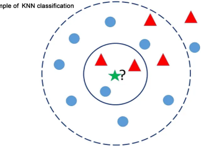
Figure 2. A diagram to show the work of NN in general. One test data point (a star in the center) should be classified either to the class of circles or to the class of triangles. The distance from this test data point to all the training data points are computed and its class membership is determined with the closest data points. As in this Figure, the test point is predicted to be in class of circles.

which is a classical activation function commonly used in classical neurons.

Following the same principle as in [3-5], this current study chooses two related quantum nearest neighbor algorithms [2, 6] and uses a simple dataset to demonstrate how they work, reveal their quantum nature, and compare their performances in detail using IBM’s quantum simulator [7].

2 METHODS

We outline the two algorithms from [2, 6] used in the current study. Each training data point is represented as n features

(

1, 2, ,

)

p p p

n

v v  v and its class label cp, where p=1, 2,,N is an index of the point in a training dataset and c∈

{

1, 2,,d

}

. Each training data point is expressed as a quantum state of

1 2

, , , , ,

p p p p p p

n

v c = v v  v c . The test data point is represented as x = x1,x2,,xn and the whole

train-ing data points are super-positioned as 1 2

1

, , , ,

p p p p n p

T v v v c

N

=

∑

_ _.

2.1. One Quantum Nearest Neighbor Algorithm from [2]

This algorithm is the quantum version of the classical weighted nearest neighbor algorithms and is inspired from the quantum associative memory in [8]. The idea is to super position all the training data points into one quantum state and then compute the Hamming distance of each training point to the test point into the amplitude of each training point in superposition. After this, measuring the class qubit re-veals the appropriate class with highest probability. Here is an outline of the algorithm.

Step one: superposition all training points into one quantum state

1 2

1

, , , ,

p p p p n p

T v v v c N

=

∑



Step two: add one ancilla qubit to this state

0 1 2 1 2

1

, , , _n; p, p, , _np, p;0

p

x x x v v v c N

ψ =

∑

 

(5)

(

)

1 1 2 1 2

1 1

, , , ; , , , , 0 1

2

p p p p

n n

p x x x v v v c

N

ψ =

∑

_ _ ⊗ +

Step four: to get the Hamming distance, apply X gate the x state and CNOT to x v, with x is

the control and v is the target

( )

(

)

(

)

2 1

1 2 1 2

1

,

1 1

, , , ; , , , , 0 1

2

p k k k k

p p p p

n n

p

X x CNOT x v N

x x x d d d c

N

ψ = ψ

= ⊗ +

∏

∑

 

Step five: apply the unitary operator π 2

e i nH

U = − , 1 1 1

( )

2

z

k c

c

H _σ _ σ

  ⊗ ⊗

+ = ⊗

∑

to add the Hamming distance p k

d of each training point vp = v₁p,v₂p,,v_np . The state after this

opera-tion is

( )

π _, 2

3 2 1 2 1 2

π _, 2

1 2 1 2

1

e , , , ; , , , , ;0

2

e , , , ; , , , , ;1

p H

i d x v

p p p p n

n n

p

i d x v _p _p _p _p n

n n

U x x x d d d c

N

x x x d d d c

ψ ψ − = = +

∑

   

where d_H

(

x v, p

)

is the Hamming distance between vp and x .

Step six: apply another Hadamard gate on the ancilla qubit

( )

4 3

1 2 1 2

1 π

cos , , , , ; , , , , ;0

2 π

sin , , , , ; , , , , ;1

2

p p p p p

H n n

p

p p p p p

H n n

H

d x v x x x d d d c

n N

d x v x x x d d d c

n

ψ = ψ

           =  +

∑

   

Step seven: from step six, it is clear that if the test point is close to the training points then we have a higher probability to measure the ancilla qubit in the state 0 , otherwise we should see it in the state 1 . The probability of getting 0 is

( )

₀ 1 _cos2 π

( )

_,

2

p

a H

p

P d x v

n N   = _ _  

∑

At this point of time, there are two paths to take. The first way is to take a “K _{all” approach by} as-signing the class of training points that are on average closer to the test point. The second is measure the class qubit and retrieve the neighbors with a probability weighted by their distance and choose a class from this pool of training points.

Following the first path, we need to measure the class qubit. To better show the different classes ap-pearing weighted by their distance to the test point,

ψ

4 is rewritten as

( )

4 1

1 2 1 2

1

π

cos , , , , ; , , , , ;0

2 π

sin , , , , ; , , , , ;1

2

d c

l l l l l

H n n

l c

l l l l l

H n n

c N

d x v x x x d d d c

n

d x v x x x d d d c

(6)

https://doi.org/10.4236/ns.2018.103010 92 Natural Science The probability of measuring a class c∈

{

1, 2,,d

}

conditioned on measuring the ancilla qubit in

0 is

( )

1

_{( )}

_cos2 π

( )

_,

0 2

l H l c

P c d x v

NP ∈ n

 

= _ _

 

∑

Following the second path, the test point is assigned the class that is in the majority of its nearest neighbors.

2.2. One Quantum Nearest Neighbor Algorithm from [6]

Inspired by the algorithm introduced in section 2.1, a quantum KNN algorithm is proposed in [6]. In addition to the well-known parameter K, it also requires another parameter t as we will explain next.

Steps one and two are the same as those outlined in section 2.1. Step three:

( )

(

)

1 0

1 2 1 2

1

,

1

, , , ; , , , , ;0

p k k k k

p p p p p p p

n n

p

X x CNOT x v N

d d d v v v c

N

ψ = ψ

=

∏

∑

 

Here the CNOT gate uses v as control and x as target, and as a result the meaning of the d_kp is

reversed, i.e., if two bits are the same then d_kp =1, otherwise d_kp =0. The reason for this reversion is ex-plained in the next step.

Step four: compute the Hamming distance with 1 , 2, ,

p p p

n

d d  d and label the test point according to

a threshold value t. This operation can be done with this unitary operator U:

2 1 1 2 1 2

1 2 1 2

1

, , , ; , , , , ;1

, , , ; , , , , ;0

p p p p p p p

n n

p

p p p p p p p

n n

p

U d d d v v v c

N

d d d v v v c

ψ ψ ∈Ω ∉Ω = = +

∑

   

where Ω_{is a set that contains indexes}_p_{with Hamming distance between} p

v and x ≤t.

Recall that the meaning p k

d is reversed, so the Hamming distance ≤t implies p i

id ≥ −n t

∑

. If K is chosen according to 1

2k− ≤ ≤n 2k, and let l=2k −n, then the condition Hamming distance ≤ t can be

rewritten as

p i

id + ≥ + −l n l t

∑

implies

∑

_id_ip+ + ≥l t 2k

From this inequality, if the initial a= +l t, then the condition of Hamming distance ≤ t can be de-termined by whether the sum of p

i id +a

∑

overflows or not.

Step five: measuring the ancilla qubit in the state of 1 can find the training points whose Hamming distance is less than t. In this algorithm there are two parameters, K and t, to select.

3 RESULTS

To compare the two classifiers from [2, 6] on a fair base, we only evaluate them by the nearest neigh-bors they select rather than the final classification results they produce, since this step is the most critical before a final classification is rendered and can be compared straightforwardly.

3.1. Dataset for Comparing the Two Algorithms

(7)

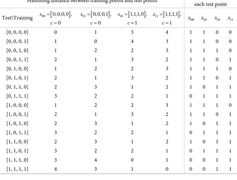
https://doi.org/10.4236/ns.2018.103010 93 Natural Science four particular numbers of them as training points with the first two training points in class 0 and second two in class 1 (Table 1). Furthermore, in order to establish a benchmark to compare the two quantum classifiers in section 2, we choose K = 2 and find the nearest neighbors for each test point manually based on the Hamming distance, which provide the best possible results (Table 1).

3.2. Performance of the First Classifier in Section 2.1

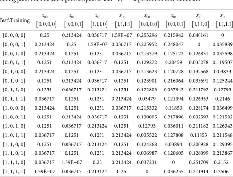
According to the probability formula in Step six in section 2.1, we calculate the theoretical probability of observing each test point and each training point when measuring the ancilla qubit in state 0 in

Ta-ble 2. Since there are four training points, the maximum probability for a test point to be seen together with a training point is 0.25. The execution of this algorithm on IBM’s quantum simulator produces the observed probabilities that match the theoretical ones very well (Table 2 and Figure 3).

[image:7.595.57.539.368.732.2]

Each entry in Table 2 represents the theoretical or the experimental probability of observing one test point and one training point together when measuring ancilla qubit in state 0 . To render a better illu-stration of these two ways of computing their probabilities, we plot them in curves in Figure 3 and we

Table 1.This table contains two sub tables. On the left is a sub table for Hamming distances between test points and training points. On the right is a sub table for the nearest neighbors of each test point selected by the Hamming distance and when K = 2, where 1 means a nearest neighbor, 0 means otherwise. This sub table displays the best possible results which will be used as a benchmark to compare the two algorithms in the next two sections.

Hamming distance between training points and test points Nearest neighbors for _{each test point}

Test\Training 00

[

0, 0, 0, 0 ,

11 1,1,1,1 ,

1

x

c =

= x00 x01 x10 x11

[0, 0, 0, 0] 0 1 3 4 1 1 0 0

[0, 0, 0, 1] 1 0 4 3 1 1 0 0

[0, 0, 1, 0] 1 2 2 3 1 1 1 0

[0, 0, 1, 1] 2 1 3 2 1 1 0 1

[0, 1, 0, 0] 1 2 2 3 1 1 1 0

[0, 1, 0, 1] 2 1 3 2 1 1 0 1

[0, 1, 1, 0] 2 3 1 2 1 0 1 1

[0, 1, 1, 1] 3 2 2 1 0 1 1 1

[1, 0, 0, 0] 1 2 2 3 1 1 1 0

[1, 0, 0, 1] 2 1 3 2 1 1 0 1

[1, 0, 1, 0] 2 3 1 2 1 0 1 1

[1, 0, 1, 1] 3 2 2 1 0 1 1 1

[1, 1, 0, 0] 2 3 1 2 1 0 1 1

[1, 1, 0, 1] 3 2 2 1 0 1 1 1

[1, 1, 1, 0] 3 4 0 1 0 0 1 1

(8)

[image:8.595.62.536.162.522.2]

Table 2. This table contains the probabilities computed from the theory of the algorithm in section 2.1 in the left sub table and the actual observed probabilities when running the algorithm on IBM’s simulator with shots = 8192 in the right sub table.

Theoretical probability of observing each test point and each training point when measuring ancilla qubit in state 0

Observed probability when running the algorithm on IBM’s simulator

Test\Training

_[

00

11

1,1,1,1

x =

[0, 0, 0, 0] 0.25 0.213424 0.036717 1.59E−07 0.253296 0.215942 0.040161 0 [0, 0, 0, 1] 0.213424 0.25 1.59E−07 0.036717 0.225952 0.248047 0 0.035889 [0, 0, 1, 0] 0.213424 0.1251 0.1251 0.036717 0.213379 0.125122 0.126831 0.037598 [0, 0, 1, 1] 0.1251 0.213424 0.036717 0.1251 0.129272 0.20459 0.035278 0.119507 [0, 1, 0, 0] 0.213424 0.1251 0.1251 0.036717 0.213623 0.120728 0.132568 0.03833 [0, 1, 0, 1] 0.1251 0.213424 0.036717 0.1251 0.123901 0.216064 0.033691 0.125244 [0, 1, 1, 0] 0.1251 0.036717 0.213424 0.1251 0.122803 0.037842 0.211792 0.12793 [0, 1, 1, 1] 0.036717 0.1251 0.1251 0.213424 0.03479 0.121094 0.126953 0.2146 [1, 0, 0, 0] 0.213424 0.1251 0.1251 0.036717 0.215332 0.11853 0.128174 0.036499 [1, 0, 0, 1] 0.1251 0.213424 0.036717 0.1251 0.130005 0.217896 0.032593 0.121582 [1, 0, 1, 0] 0.1251 0.036717 0.213424 0.1251 0.12793 0.036011 0.211182 0.126343 [1, 0, 1, 1] 0.036717 0.1251 0.1251 0.213424 0.035522 0.127808 0.11853 0.211548 [1, 1, 0, 0] 0.1251 0.036717 0.213424 0.1251 0.124268 0.03894 0.200928 0.129395 [1, 1, 0, 1] 0.036717 0.1251 0.1251 0.213424 0.036987 0.120605 0.126099 0.213867 [1, 1, 1, 0] 0.036717 1.59E−07 0.25 0.213424 0.037231 0 0.251709 0.21521 [1, 1, 1, 1] 1.59E−07 0.036717 0.213424 0.25 0 0.036255 0.211914 0.25061

can visually see that the two results match perfectly, giving the random nature of reading these values on a quantum simulator.

For the sake of comparing this classifier with the one in section 2.2, we set K = 2 in this experiment to satisfy the condition of 1

2k− ≤ ≤n 2k here n = 4, as required by the classifier in section 2.2. The algorithm

in section 2.1 offers to two different path ways to get the final classification based on the measured proba-bilities, while the one in section 2.2 produces the final classification based on whether or not there is an overflow in the addition of the Hamming distances to the quantum register that holds the value of a, which depends on the value of t. For this reason, we choose to compare these two classifiers based on the nearest neighbors they generate rather than the final predication. To select the nearest neighbors for the algorithm in section 2.1, for each test point we choose the two training points with top two probabilities as nearest neighbors since K = 2. From the theory shown in Table 2, there are two equal probabilities in some cases. If this happens, we choose three nearest neighbors instead of two.

(9)

[image:9.595.58.543.72.457.2]

Figure 3. This figure plots the actual numerical values in Table 2 to visualize how closely the expe-rimental results match the theoretical results. The x-axis represents the 16 test points as defined in

Table 1.

3.3. Performance of the Second Classifier in Section 2.2

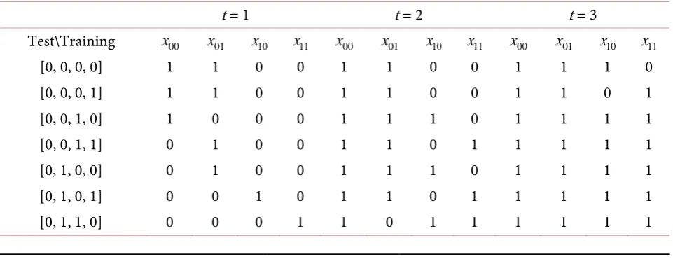
Since n = 4, we choose K = 2 to satisfy the condition 2k−1≤ ≤n 2k_{. Let}_t_{= 1, 2, 3 respectively and the} algorithm finds the nearest neighbors accordingly when running it on IBM’s quantum simulator (see Ta-ble 4). Recall from section 2.2 that the selection of nearest neighbors in this algorithm is to check if there is an overflow or not when we add the Hamming distances to the quantum register that hold the value of a(t). So only in this sense, the nearest neighbor selection process in this algorithm is deterministic.

4. CONCLUSIONS

(10)

[image:10.595.60.541.556.741.2]

Table 3. This table displays the nearest neighbors for each test point selected by the algorithm in section 2.1 when K = 2, where 1 means a nearest neighbor, 0 means otherwise. The results in this table match 100% with the best possible results in Table 1.

c=1

[0, 0, 0, 0] 1 1 0 0

[0, 0, 0, 1] 1 1 0 0

[0, 0, 1, 0] 1 1 1 0

[0, 0, 1, 1] 1 1 0 1

[0, 1, 0, 0] 1 1 1 0

[0, 1, 0, 1] 1 1 0 1

[0, 1, 1, 0] 1 0 1 1

[0, 1, 1, 1] 0 1 1 1

[1, 0, 0, 0] 1 1 1 0

[1, 0, 0, 1] 1 1 0 1

[1, 0, 1, 0] 1 0 1 1

[1, 0, 1, 1] 0 1 1 1

[1, 1, 0, 0] 1 0 1 1

[1, 1, 0, 1] 0 1 1 1

[1, 1, 1, 0] 0 0 1 1

[1, 1, 1, 1] 0 0 1 1

Table 4. This table displays the nearest neighbors for each test point selected by the algorithm in section 2.2 when K = 2 and t = 1, 2, 3, respectively, where 1 means a nearest neighbor, 0 means oth-erwise. Compared with the best possible results in Table 1, when t = 1, there are 29 mismatches, t = 2 match perfectly, t = 3 have 16 mismatches. The algorithm is run on IBM’s simulator with 1000 shots. Nearest neighbors for each test point selected by running the algorithm in section 2.2 on IBM’s simulator

t = 1 t = 2 t = 3

Test\Training x00 x01 x10 x11 x00 x01 x10 x11 x00 x01 x10 x11

[0, 0, 0, 0] 1 1 0 0 1 1 0 0 1 1 1 0

[0, 0, 0, 1] 1 1 0 0 1 1 0 0 1 1 0 1

[0, 0, 1, 0] 1 0 0 0 1 1 1 0 1 1 1 1

[0, 0, 1, 1] 0 1 0 0 1 1 0 1 1 1 1 1

[0, 1, 0, 0] 0 1 0 0 1 1 1 0 1 1 1 1

[0, 1, 0, 1] 0 0 1 0 1 1 0 1 1 1 1 1

(11)

Continued

[0, 1, 1, 1] 1 0 0 0 0 1 1 1 1 1 1 1

[1, 0, 0, 0] 0 1 0 0 1 1 1 0 1 1 1 1

[1, 0, 0, 1] 0 0 1 0 1 1 0 1 1 1 1 1

[1, 0, 1, 0] 0 0 0 1 1 0 1 1 1 1 1 1

[1, 0, 1, 1] 0 0 1 0 0 1 1 1 1 1 1 1

[1, 1, 0, 0] 0 0 0 1 1 0 1 1 1 1 1 1

[1, 1, 0, 1] 0 0 1 1 0 1 1 1 1 1 1 1

[1, 1, 1, 0] 0 0 1 1 0 0 1 1 1 0 1 1

[1, 1, 1, 1] 0 0 1 1 0 0 1 1 0 1 1 1

requires the choice for K and has an additional parameter t to set up and as a result, its performance heav-ily depends on the value of t. Both have their runtime independent of dataset size N but dependent on the number of features n for each data point, which offers a huge advantage in processing big data [2, 6]. The quantum nature of these two classifiers is better revealed when testing them on a manageable dataset pro-posed in this study. The classifier from [2] demonstrates its perfect results to match the best possible re-sults, in contrast, the results of second one from [6] vary according to different values of the parameter t, assuming both choose K = 2.

In addition to the papers that we have cited in this paper so far, we are also inspired by and have be-nefited from reading these ones [9-17].

ACKNOWLEDGEMENTS

We thank IBM Quantum Experience for use of their quantum computers and simulators.

REFERENCES

1. Biamonte, J., Wittek, P., Pancotti, N., Rebentrost, P., Wiebe, N. and Lloyd, S. (2017) Quantum Machine Learn-ing. Nature, 549, 195-202. https://doi.org/10.1038/nature23474

2. Schuld, M., Sinayskiy, I. and Petruccione, F. (2014) Quantum Computing for Pattern Classification. Pacific Rim International Conference on Artificial Intelligence, 208-220. https://doi.org/10.1007/978-3-319-13560-1_17 3. Hu, W. (2018) Empirical Analysis of a Quantum Classifier Implemented on IBM’s 5Q Quantum Computer.

Journal of Quantum Information Science, 8, 1-11.

4. Hu, W. (2018) Empirical Analysis of Decision Making of an AI Agent on IBM’s 5Q Quantum Computer. Natu-ral Science, 10, 45-58. https://doi.org/10.4236/ns.2018.101004

5. Hu, W. (2018) Towards a Real Quantum Neuron. Natural Science, 10, 99-109.

6. Ruan, Y., Xue, X.L., Liu, H., Tan, J.N. and Li, X. (2017) Quantum Algorithm for K-Nearest Neighbors Classifi-cation Based on the Metric of Hamming Distance. International Journal of Theoretical Physics, 56, 3496-3507. https://doi.org/10.1007/s10773-017-3514-4

7. IBM. Quantum experience. http://www.research.ibm.com/quantum

8. Trugenberger, C.A. (2001) Probabilistic Quantum Memories. Physical Review Letters, 87, 067901. https://doi.org/10.1103/PhysRevLett.87.067901

(12)

https://doi.org/10.4236/ns.2018.103010 98 Natural Science Physical Review A, 94, 022342. https://doi.org/10.1103/PhysRevA.94.022342

10. Schuld, M., Sinayskiy, I. and Petruccione, F. (2015) Simulating a Perceptron on a Quantum Computer. Physics Letters A, 379, 660-663. https://doi.org/10.1016/j.physleta.2014.11.061

11. Schuld, M., Sinayskiy, I. and Petruccione, F. (2014) The Quest for a Quantum Neural Network. Quantum

In-formation Processing, 13, 2567-2586. https://doi.org/10.1007/s11128-014-0809-8

12. Schuld, M., Sinayskiy, I. and Petruccione, F. (2014) Quantum Walks on Graphs Representing the Firing Patterns of a Quantum Neural Network. Physical Review A, 89, 032333. https://doi.org/10.1103/PhysRevA.89.032333 13. Schuld, M., Sinayskiy, I. and Petruccione, F. (2014) An Introduction to Quantum Machine Learning.

Contem-porary Physics, 56, 172-185. https://doi.org/10.1080/00107514.2014.964942

14. Schuld, M., Fingerhuth, M. and Petruccione, F. (2017) Implementing a Distance-Based Classifier with a Quan-tum Interference Circuit. A Letters Journal of Exploring the Frontiers of Physics, 119, 60002.

https://doi.org/10.1209/0295-5075/119/60002

15. Cai, X.-D., Wu, D., Su, Z.-E., Chen, M.-C., Wang, X.-L., Li, L., Liu, N.-L., Lu, C.-Y. and Pan, J.-W. (2015) En-tanglement-Based Machine Learning on a Quantum Computer. Physical Review Letters, 114, 110504.

https://doi.org/10.1103/PhysRevLett.114.110504

16. Lloyd, S., Mohseni, M. and Rebentrost, P. (2013) Quantum Algorithms for Supervised and Unsupervised Ma-chine Learning. arXiv preprint arXiv:1307.0411.