Cascade Algorithm Revisited

Cascade Algorithm Revisited

Tadao Takaoka

, Kiyomi Umehara

_{Department of Computer Science}

University of Canterbury

Christchurch, New Zealand

∗∗

_{Hitachi Laboratory}

Tokyo, Japan

January 1990, revised November 2013

Abstract

We revisit the cascade algorithm for the all pairs shortest path (APSP) problem. The operation on the distace data is limited to the triple oper-ation of min{a, b+c}. The best known complexity on this model isn3

by Floyd’s algorithm. The cascade algorithm takes 2n3 opearations. We first improve this bound ton3, that is, on a par with Floyd’s algorithm. Then we implement the improved version on a mesh computer and achieve 3n−2 communication steps.

1

Introduction

We consider a directed graphG = (V, E) where V ={1,2, ..., n} is the set of vertices given by integers andE is the set of edges given by pairs of integers. We associate a non-negatice edge costdijwith edge (i, j). By

setting dij to ∞when pair (i, j) is not inE, we have an (n, n) square

matrix D ={dij}. The seuqence of edges (i, k1)(k1, k2)...(km, j) where

m≥1 is a path from ito jof lengthm+ 1. Note that the path is just edge (i, j) when m = 0. The cost of the path is the sum of the costs of edges in the path. The cost of the shortest path from itoj is called the shortest distance from i to j. The all pairs shortest path (APSP) problem is to compute the shortest paths fromito j for all pairs (i, j). Letd∗ijbe the shortest distance fromitoj, andD

∗

={d∗ij}. W will show

how to compute D∗ from the given matrixD. That is, we compute the shortest distance matrixD∗fromD. D∗is called the closure ofD. The shortest paths fromitojfor all (i, j) can be computed as by-product in the process of computingD∗. Hence we mainly focus on how to compute

D∗. We assume that the diagonal elements ofD are 0.

Note that previously computeddij are used later in the computation in

this algorithm.

Classical cascade algorithm

{forward process}

fori:=1tondo fori:=1tondo begin c:=∞;

fork:=1tondoc:=min{c, dik+dkj}

dij:=c

end

{backward process}

fori:=ndownto1do for i:=ndownto1do begin c:=∞;

fork:=ndownto1doc:=min{c, dik+dkj}

dij:=c

end

fori:=1tondo fori:=1tondod∗ij:=dij

In the forward processi, jandksweep in increasing order, whereas in the backward process they sweep in decreasing order. Let us call the op-eration min{a, b+c}the triple operation wherea, bandcare non-negative real numbers. In this paper we measure the complexity of algorithms by the number of triple operations executed. In the above cascade algorithm, the number of triple operations is obviously 2n3. In contrast, the follow-ing Floyd’s algorithm [3] computesD∗withn3 _{triple operations.}

Floyd’s algorithm fork:=1tondo

fori:=1tondo for j:=1tondo dij:=min{dij, dik+dkj}

fori:=1tondo fori:=1tondod∗ij:=dij

Because of its simplicity and less complexity, Floyd’s algorithm seems to be superior to the cascade algorithm and the latter seems to have been forgotten.

In the next section we improve the number of triple operations in the cascade algorithm ton3. Johnson [7] showed that if only comparisons and additions are used in a straight-line program to solve the APSP problem, we need 2n(n−1)(n−2) operations. We show that both of Floyd’s algorithm and the cascade algorithm are optimal in this computational model. A straight-line program has no branching on the processed data. We count only operations on distance data, not on control variables. In Sections 3 and 4, we give a correctness proof and analysis of the algorithm. In Section 5, we further modify the improved cascade algorithm and show how to design a VLSI circuit for the modified cascade algorithm. The circuit is ofO(n2) aize and takesO(n) time. This is an improvement of the VLSI implementation by Sinha, et. al [?], which is ofO(n2_{) size}

amd takesO(nlogn) time andO(n2) propagaton time.

case. The expected computing time of the improved version isO(n2.5).

2

Improved cascade algorithm

A careful review of the proof of the algorithm in [4] brings us an improve-ment by limiting the sweeping range of the control variablekin both the forward and backward processes in the following way.

Improved cascade algorithm

{forward process}

fori:=1tondo forj:=1tondo begin c:=dij;

fork:=1tomin{i, j} −1doc:=min{c, dik+dkj}

dij:=c

end

{backward process}

fori:=ndownto1do forj:=ndownto1do begin c:=dij;

fork:=ndowntomin{i, j}+ 1doc:=min{c, dik+dkj}

dij:=c

end

fori:=1tondo fori:=1tondod∗ij:=dij

We give the proof for the correctness in the next section.

3

Correctness

Let us denote the path (i, k1)(k1, k2)...(km, j) by vertices (i, k1, ..., km, j).

Definition 1 The path(i, k1, ..., km, j)is

(1) an up sequence, ifi < k1< ... < km< j,

(2) a down sequence, ifi > k1> ... > km> j,

(3) a valley sequence, ifk`< iandk`< j)for all`, or

(4) a hill sequence, ifk`> i andk`> j)for all`.

We note that all verices in each of the above sequences are distinct. That is, we only consider simple paths. We use the fact thatdij is

com-puted later (earlier) thandi0_j0 is ifi0< iandj0< jin the forward process

(backward process). Whenm= 1, that is, the path has only two edges, we call (3) a short valley sequence and (4) a short hill sequence.

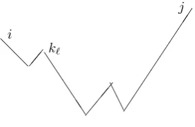
Lemma 1 If the shortest path from i to j, (i, k1, ..., km, j), is a valley

sequence, the value ofdijgives the shortest distance fromitojat the end

of the forward process.

Proof. Let the path length is the number of edges in the given path. Proof is by induction on the path length. To prove the basis we assume a short valley sequence (i, k1, j) is the shortest path form= 1. Then edge

(i, k1) and edge (k1, j) are the shortest paths fromitok1and fromk1 to j. Since they are the shortest distances and k1 <min{i, j}, dij is given

i

k1

j

@

@

@

@

@

@% %

% %

% %

% %%

j k1

i k1

Figure 1: Short valley sequence and sweeping bykto capturesk1.

Now letk`= max{k1, ..., km}, (m >1), that is, the path length ism+1.

Then the sequence (i, k1, ..., k`) and (k`, ..., km, j) form valley sequences,

or single edges when`= 1 or`=m. By the induction hypothesis as their path lengths are up tom, we can assumedik` anddk`jgive the shortest

distances fromitok`and the shortest distance fromk`to j. Sincek`<

min{i, j},dijis given bydik`+dk`j. See Figure 2.

i

k`

j

@

@

% %%A

A

J

J

J

J J %%

Figure 2: Long valley sequence

If the algorithm computes the shortest distance fromitojindij, we

assume a hypothetical edge (i, j) with costdij. We say the shortest path

Now we modify the forward process in the following way.We call the modified process the long forward process (LFP). In contrast, we call the original forward process the short forward process (SFP). The naming comes from the distance of sweeping by the control variablek.

{Long forward process}

fori:=1tondo forj:=1tondo begin c:=dij;

fork:=1tomax{i, j} −1doc:=min{c, dik+dkj}

dij:=c

end

Lemma 2 If the shortest path fromi toj, (i, k1, ..., km, j), is one of the

following three, the value ofdij gives the shortest distance fromitojat

the end of the long forward process. We define an extended valley sequnce as a vally sequence preceded by an initial down sequence or followed by a final up sequence. An extended hill sequence is defined similarly.

(1) Extended valley sequence (2) Up sequence

(3) Down sequence.

Proof. For (1), let us assume an extended valley sequence from i to

j such that i < j. Let k be the minimum of vertices on the final up-sequence that is greater thani. The subsequence fromitok is a valley sequence covered by Lemma 1, which reduces the valley sequence into a single edge and forms an up-sequence with the sequence fromktoj. Since the vertices fromkto jappear in increasing order in the algorithm, the computational process is the same as for an up-sequence in (2). The case ofi > jis symmetric.

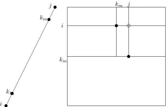
We prove (2) by induction. To prove the basis we assume an up-sequence is an edge(i, j). Obviouslydijgives the shortest distance at the

end of the long forwards process. Assume by induction thatdikmgives the

shortest distance fromitokmafter the LFP. Then the shortest distance

dijfromitojis given bydikm+dkmj, sincekm<max{i, j}. See Figure

3. Note that the distances on the path (i, k1, ..., km, j) are computed in

the order ofdik1, ..., dikm, dij. The proof for (3) is is similar and seen from

Figure 4. Note that the shortest distances on the path (i, k1, ..., km, j) are

computed in the order ofdkmj, ..., dk1j, dij.

Now we call the original backward process the long backward process (LBP), and define the short backward process (SBP) in the following.

{Short backward process}

fori:=ndownto1do forj:=ndownto1do begin c:=dij;

fork:=ndowntomax{i, j}+ 1doc:=min{c, dik+dkj}

dij:=c

j km

km

i t d

t

t i

t k1

t km

t j

Figure 3: Working on the up-sequence

j km

km

i

t

t d

A

A

A

A

A

A

A

A

A

A

A

A

A

A

A

A

t i

t k1

t km

t j

Lemma 3 If the shortest path from i to j, (i, k1, ..., km, j), is a hill

se-quence, the value of dij gives the shortest distance fromitoj at the end

of the short backward process.

Proof. Similar to Lemma 1.

Lemma 4 If the shortest path fromi toj, (i, k1, ..., km, j), is one of the

following three, the value ofdij gives the shortest distance fromitojat

the end of the long backward process.

(1) Extended hill sequnce (2) Up sequence

(3) Down sequence.

Proof. Similar to Lemma 2.

Note that in Lemma 3 and Lemma 4, we execute the SBP and LBP in isolation, not in conjunction with a forward process. Now we define by (P, Q) the execution of the processesP andQin this order. The first case of the following theorem is the improved cascade algorithm we mentioned earlier in the paper.

Theorem 1 The execution of each of (SFP, LBP) and (SBP, LFP)

com-putes indij the shortest distance fromitoj.

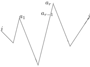
proof. We give a proof for (SFP, LBP). The other proof is similar. Now we reduce the shortest path fromitoj, (i, k1, ..., km, j) to (i, a1, ..., ar, j)

by reducing the maximal valley parts into edges. See Figure 5. Vertices

a1, ..., arare such that the sub-sequence fromaktoak+1forms a maximal

valley sequence, an up-sequence or a down-sequence. A valley sequece is maximal if it is a valley sequence and it is not a part of a larger valley sequence. The sequence (i, a1, ..., ar, j) is in general a composite of an

up-sequence followed by a down-up-sequence. Obviously the reduced up-sequence (i, a1, ..., ar, j) is an extended hill sequence, an up-sequence or a

down-sequence. The SFP computes the shortest distance between any pair of vertices in the reduced sequence. By assuming hypothetical single edges with distances obtained in the SFP between these pairs, we see that the LBP computes the shortest distances fromitoj.

i

a1 ar−1

ar j @ @ L L L L L L L L L L L L L L L

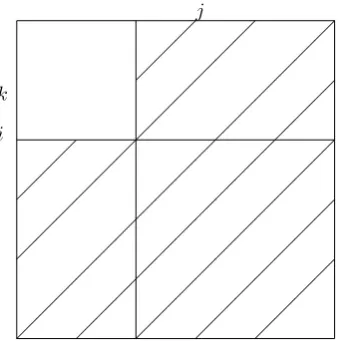
k

i

j

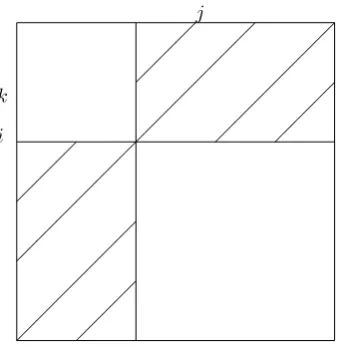
Figure 6: Analysis of SFP

4

Analysis

We count the number of triple operatons in the improved cascade algo-rithm. Note that a triple operation consists of one comparison and one addition. In the SFP, the number is measured by the summation of the hatched part in Figure 6. The number of triple operationd is given by

F= 2Σn

i=1(i−1)(n−i) = 2(n+ 1)Σin=1i−2Σni=1i2−2n2

= (n+ 1)n(n+ 1)−(2/6)n(n+ 1)(2n+ 1)−2n2

= (1/3)n3_−n2_{+ (2/3)n}

We analyze the LBP by using the LFP, since the two are computaion-ally symmetric. See Figure 7. The number of triple operations is

B=F+ Σni=1[(n−i) 2

−(n−i)] =F+ (1/3)n3−n2+ (2/3)n

Hence the total number of triple operations is given by F +B = n3−

3n2_{+ 2n. In this analysis we changed the LFP slightly so thatkskips the}

casesk=iifi < jandk=jifi > j. In Theorem 2, this changed version is used.

In thek-th iteration of the Floyd algorithm, we can avoid updating the value ofdijin the k-th row and column, and also we can avoid updating

diagonal elements. In this version, the Floyd algorithm takesn(n−1)(n−

2) triple operations, which is equal to the above figure. Also in Johnson, is is shown that 2n(n−1(n−2) operations are required if the computational model is limited to the one introduced in Introduction. Hence we have

Theorem 2 The improved cascade algorithm is optimal in the

k

i

j

Figure 7: Analysis of LFP

Now we try to speed up the algorithm for acyclic graphs. We suppose that the given graph is acyclic and vertices are topologically sorted, that is, if (i, j)∈Etheni < j. Then the shortest paths are all up sequences. Hence the shortest distances are obtained afte the LFP. But we can speed up the LFP even more in the following.

{Modified long forward process, MLFP}

fori:=1tondo forj:=i+ 1tondo begin c:=dij;

fork:=i+ 1toj−1doc:=min{c, dik+dkj}

dij:=c

end

An easy calculation reveals that the number of triple operations is (1/6)n(n−1)(n−2). This figure is equal to that for the Floyd algorithm if it is applied to an upper triangle matrix for an acycle graph.

If vertices are toplogically sorted in reverse order, the following algo-rithm computes the shortest distances.

{Modified long backward process}

fori:=ndownto1do forj:=i−1downto1do begin c:=dij;

fork:=i−1downtoj+ 1doc:=min{c, dik+dkj}

dij:=c

end

Note that MLFP and MLBP are computationally symmetric. The former works on the upper-right triangle and the latter on the lower-left triangle of the matrix.

se-quence and a down sese-quence respectively.

proofLet(i, k1, ..., km, j)be the up sequence that gives shortest path from

i to j. From induction we can assume the shortest distance for the up sequence(i, k1, ..., km)is computed indikm. Sincei < km< j, the MLFP

captures the shortest path successfully. Similarly the MLBP computes the shortest distance for the down sequence.

From discussions from the previous sections, we have the following theorem useful for VSLI implementation.

Theorem 3 The sequential execution of (SFP, SBP, MLFP, MLBP) in

this order computes all shortest distances. The number of triple operations isn(n−1)(n−2), which is optimal in the same computational model as in the previous section.

ProofThe SFP reduces the shortest path fromitoj, (i, k1, ..., km, j), to

(i, a1, ..., ar, j)as described in Theorem 1. This is:

(1) an up-sequence, (2) a down sequence, or

(3) an up sequence followed by a down sequence, that is, extended hill sequence.

In case of (3), the SBP reduces it into an up sequence or down se-quence. The MFLP computes the shortest distance for the up sequences and the MLBP computes the shortest distances for the down sequences, from Lemma 5. The analysis is straightforward.

5

Approach by forward process only

Lemma 6 LFP reduces the shortest path sequence from itoj to an up-sequence, a down up-sequence, or an extended hill sequence. LBP reduces the shortest path sequence fromitojto an up-sequence,a down-sequence, or an extended valley sequence.

Proof. LFP reduces an extended valley sequence from itoj to an edge going up ifi < j and going down ifi > j. The latter half of the lemma is symmetric.

Let us square the given distance matrix three times based on the LFP given in the previou sections. Then we have:

Theorem 4 Two LFP squarings and a full squaring solve the APSP prob-lem. The number of triple operations is2n3_−6n2_{+ 4n.}

ProofThe first squaring reduces the shortest paths into an up-sequence, down-sequence or extended hill sequence. The second squaring reduces the up-sequences and down-sequences into single edges, leaving only short hill sequences. The last squaring computes shortest distances for those short hill sequences. For the analysis, the number of triple operations is 3((2/3)n3−2n2+ (4/3)n) = 2n3−6n2+ 4n.

mesh architecture. We call the first the buffer method and the second the in-place method. We begin with the buffer method.

The input is the skewed and reversed matrix fed into the mesh from left and the same matrix skewed and reversed vertically, fed from above vertically. Thus the mesh architecture square the given distance matrix with cascading. Ignoring the constant terms, direct implementation of matrix multiplication on VLSI takes 3n steps. We showed three LFP multiplications solve APSP. If we use wrap around connection APSP can be solved in 5n steps. As Umehara points out, if we feed the mesh from four directions, and take the final result from the upper triangle and lower triangle, this reduces to 4n(Umehara’s Masters thesis at Ibaraki Univer-sity, 1990). On the other hand Bae, Shinn and Takaoka invented a mesh algorithm for matrix multiplication that takes 3.5n steps. That can be applied to our APSP problem, resulting in 3.5n steps on a VLSI, which is on a par with the best bound by Takaoka and Umehara in 1992.

LetRijbe the accumulator incell(i, j). Letdijandd0ijbe the distance

data in the input buffer, the former go from left to right and the latter from top to down. The algorithm atcell(i, j) is described below.

Algorithm for cell(i, j) for LFP

1. Receive the new values ofdandd0 from left and up. 2. Ifdijarrives atcell(i, j), performdij:=Rij(Data release).

3. Ifd0ijarrives atcell(i, j), performd

0

ij:=Rij(Data release).

4. At timei+j+k−2,Rij:=min{Rij, dik+d0kj}is performed

Atcell(i, j), the triple operationR:=min{R, d+d0}is executed using

R,d,d0 registers. In step 4,i,j andkare meant to be comments. Note that ifdijord0ijdoes not arrive, thedord0value is sent unchanged to the

next cell. Also note thatRij is sent right or down before its completion

in general, that is, k sweeps from 1 to max{i, j}-1, not to n. In the last squaring, the value ofdij andd0ij released fromRij. The lastRij is

obtained by sweepingktonbeyond the release time.

Lemma 7 The distance dij arrives at cell(i, k) at time i+j+k−2.

Similarlyd0ij arrives atcell(k, j)at timei+j+k−2.

Proof. Note that the sums of two indices are equal in each column of the left buffer. The sum of those in the column that includesdij isi+j−1.

The column arrives at the left border of the mesh at i+j−1. Then to reachcell(i, k), it takes anotherk−1steps. The proof ford0ij is similar.

Lemma 8 Bothdikandd0kjarrive atcell(i, j)at the same timei+j+k−2.

Proof. In the previous lemma, change the roles ofkandj andk andi.

This lemma ensures that the the two distance data meet at the right place at the right time in the step 1 of the algorithm.

Lemma 9 Eachcell(i, j)can correctly performdij:=Rijat timei+ 2j−2

andd0ij:=Rij at time2i+j−2.

Proof. The sweeping by k stops at max{i, j} −1in LFP. The partially completed value ofcmust be consumed down stream in rowiand column

arrives atcell(i, j)ati+2j−2andd0ijarrives atcell(i, j)at2i+j−2. We

prepare control signals. Both originates at cell(1,1) at time 1. The first signal goes down at speed 1 and upon receiving, each cell sends a signal to the right at speed 1/2. The second signal is a mirror image of the first signal.

Note. Another way for the timing of data release is to prepare control signals 1 tok, and use the main diagonal for the origin of each control signal. Thek-th control signal originates atcell(k, k) at time 3k−2 and propagates right and down spending one unit of time from cell to cell. Then it propagates tocell(i, j) at time 3k−2 +i−k+j−k=i+j+k−2. Fori < j, thej-th control signal comes tocell(i, j) at timei+ 2j−2 and fori > j, thei-th control signal comes tocell(i, j) at time 2i+j−2.

Theorem 5 The algorithm is correct. It finishes atk= 5n−2.

If we perform the cascade multiplication 3 times, the first two takensteps each. The last takes 3n−2 steps, resulting in 5n−2 steps altogether. The computation of the three multiplications go in a pipe-line fashion. The input is loaded into the buffers initially. The first multiplication takes

n steps to bringd11 to the right border. The right border is connected

to the left border by wrap arounds. As soon as a datum comes to the right border, it is sent to the left border, effectively starting the second multiplication with the control signal starting atcell(1,1) again. As the values ofdij andd0ij go through the mesh in skewed forms, the data are

fed into the mesh in skewed forms after n steps. Then as soon as the second multiplication spends nsteps, the third starts with inputs again through the wrap arounds in skewed forms, taking 3n−2 steps this time.

Theorem 6 APSP can be solved on a mesh array in4n steps.

Proof We prepare skewed matrices to be fed from left, from up, from right and from down. The computation on the data from left and top can be done in the first layer and that on the data from right and down can be done in the second layer. The above described computation can stop at 4n−1 steps, the last multiplication taking 2n−1 steps. The two computations go independently in the two layers, the second computation being a mirror image of the first. The result can be obtained from the top-left triangle of the first layer and the bottom-right triangle of the second layer, spending one more step.

For the lower bound, take an example graph,G= (V, E) whereE=

{(1, n),(n,2),(2, n−1)}. Obviously the shortest distance from vertex 1 to vertexn−1 isd1,n+dn,2+d2,n−1. We have four copies ofdn,2in the input

buffers. The distancedn,2needs to traverse from its original positions to cell(1, n−1) taking 2n−2 steps. Thus ignoring constant terms, we still have the gap of 2nsteps.

References

[2] B. A. Farby, A. H. Land J. D. Murchland, The cascade algorithm for finding all shortest distances in a directed graph, Management Science 14, 19-28, 1967

[3] Floyd, R. W. Algorithm 97: Shortest path. Comm. ACM. 5,6 (June 1962), p. 345.

[4] Hu, T. C. Revised matrix algorithm for shortest paths. SIAM J. Appl. Math. 15, I (Jan. 1967), 207-218.

[5] Lakhani, G., and Dorairaj, R. A VLSI implementation of all-pair shortest path problem. Proc. 1987 International Conference on Par-allel Processing. IEEE Computer Society, 1987, pp. 207-209.

[6] Lewis, P., and Kung, S. An optimal systolic array for the algebraic path problem. IEEE Trans. Comput. C-40, 1 (Jan. 1991), 100-105.

[7] D. B. Johnson, Algorithms for shortest paths, TR-73-169, Ph. D thesis, dept of Computer Science, Cornell University, 1973 .

[8] van de Snepscheut, J. L. A. A derivation of a distributed implemen-tation of Warshall s algorithm. Sci. Comput. Programming. 7, 2 (Sept. 1986), 55-60.

[9] Tadao Takaoka: All Pairs Shortest Paths via Matrix Multiplication. Encyclopedia of Algorithms 2008