University of Warwick institutional repository: http://go.warwick.ac.uk/wrap
This paper is made available online in accordance with publisher policies. Please scroll down to view the document itself. Please refer to the repository record for this item and our policy information available from the repository home page for further information.
To see the final version of this paper please visit the publisher’s website. Access to the published version may require a subscription.
Author(s): Mark B Stewart
Article Title: Wage Inequality, Minimum Wage Effects and Spillovers Year of publication: 2011
Link to published article:
http://www2.warwick.ac.uk/fac/soc/economics/research/workingpapers/ 2011/twerp_965.pdf
Wage Inequality, Minimum Wage Effects and Spillovers
Mark B Stewart
No 965
WARWICK ECONOMIC RESEARCH PAPERS
Wage Inequality, Minimum Wage Effects and Spillovers*
Mark B Stewart University of Warwick
May 2011
Abstract
This paper investigates possible spillover effects of the UK minimum wage. The halt in the growth in inequality in the lower half of the wage distribution (as measured by the 50:10 percentile ratio) since the mid 1990s, in contrast to the continued inequality growth in the upper half of the distribution, suggests the possibility of a minimum wage effect and spillover effects on wages above the minimum. This paper analyses individual wage changes, using both a difference-in-differences estimator and a specification involving cross-uprating comparisons, and concludes that there have not been minimum wage spillovers. Since the UK minimum wage has always been below the 10th percentile, this lack of spillovers implies that minimum wage changes have not had an effect on the 50:10 percentile ratio measure of inequality in the lower half of the wage distribution.
JEL classifications: J31, J38, J08.
*
The author is grateful to the ESRC (under award RES000222611) and the Low Pay Commission for financial support and to Tim Butcher and Steve Machin for comments on an earlier version of the paper. The ASHE
data were made available by the ONS, through the LPC, and have been used by permission.
1. Introduction
The growth in wage inequality in the UK, the US and many other countries over the last 30
years is well documented. See, for example, Autor et al. (2008) for the US and Machin (2011)
for the UK and an international comparison. In the UK there has been fairly continual growth
in the 90:10 wage percentile ratio since about 1978. The increase in inequality over the period
as a whole is exhibited in both the upper and lower halves of the distribution. However an
important feature of inequality growth since the mid 1990s has been the different behaviour of
the dispersion in the upper and lower halves of the distribution. The inequality in the upper
half of the distribution (as measured by the 90:50 percentile ratio) has kept on increasing,
while that in the lower half (as measured by the 50:10 percentile ratio) has not. The latter has
been roughly flat (and falling on some measures) since about the mid 1990s.
This recent divergence in inequality paths, following roughly three decades when the paths
have been fairly similar to one-another, has led to the suggestion that the underlying
movement in inequality has been offset at the bottom end of the distribution by the impact of
the minimum wage. See Manning (2011) for a discussion of this. The UK national minimum
wage was introduced in April 1999, following a period in which there was no wage floor in
the UK. Some of its subsequent upratings have been larger than general wage growth and
some smaller, but overall the minimum wage has grown faster than the median. However
throughout the period since its introduction the UK minimum wage has been below the 10th
wage percentile. Thus an impact on the 50:10 percentile ratio would require there to have
been “spillover” or “ripple” effects on wages above the minimum. Testing for minimum wage
spillover effects can therefore throw light on these changes in wage inequality and in
particular on the recent divergent paths of inequality in the upper and lower halves of the
distribution.
Investigation of minimum wage spillover effects is also important in the context of the range
of empirical analyses conducted on the impact of the minimum wage on employment and
other outcomes based on difference-in-differences estimators with a group already slightly
above the new minimum rate used as the control group. This approach relies on the
identifying assumption that the wages of those in the control group are not affected by the rise
in the minimum wage, i.e. on the absence of wage spillovers. The approach has been used to
et al., 2009), hours (e.g. Stewart and Swaffield, 2008, Dickens et al., 2009) and second job
holding (Robinson and Wadsworth, 2007) among other outcomes.
The empirical investigation of potential minimum wage spillover effects is therefore crucial
both to the study of lower tail wage inequality and to studies of other outcomes based on a
control group from above the minimum. This paper presents an empirical investigation of
spillover effects of the introduction of the UK minimum wage and of its subsequent upratings.
The potential distributional consequences of minimum wages have long been pointed to in the
theoretical literature (Stigler, 1946), but the effect of minimum wages on the shape of the
wage distribution has received considerably less empirical attention than the effect on
employment, which has been the subject of extensive empirical investigation in many
countries. Most of the available evidence is for the US and suggests extensive spillovers. The
much smaller UK literature mostly does not find evidence of spillovers. Both are reviewed in
the next section of the paper.
This paper provides an analysis of individual wage changes. It compares the observed wage
distribution after an increase in the minimum wage with the counterfactual distribution in the
absence of the rise, estimated from the observed wage distribution before the increase, and
tests for a gap between them, constituting a spillover from the minimum wage increase. The
method used to construct this counterfactual wage distribution is of crucial importance. Two
alternative, but related, econometric approaches to constructing this counterfactual are used: a
difference-in-differences estimator for each change in the minimum and a specification that
makes use of cross-uprating comparisons. There has been considerable variation in the sizes
of upratings over the period studied here and this latter approach makes use of this variation.
Spillover effects can be expected for several reasons and under contrasting theoretical models
of the labour market. The next section discusses why spillovers may occur and then discusses
the existing evidence. Section 3 describes the empirical framework used in the paper, the
methods of estimation used and how they construct the counterfactual. Autor et al. (2010)
stress the problem of measurement error in their analysis of spillover effects. It is vitally
important for the analysis of spillovers to use as accurate data as possible. This paper uses
data from the Annual Survey of Hours and Earnings (ASHE), in which employers provide
accuracy. Section 4 describes the ASHE data used. Section 5 presents results and Section 6
conclusions.
2. Minimum wage spillovers
Minimum wage spillover effects may occur for a number of reasons. First, an increase in the
minimum raises the relative price of low-skilled labour. This may lead to a rise in the demand
for certain types of more skilled labour, depending on substitutability, and hence to increased
wages for certain types of worker already above the minimum. Second, it may lead firms to
reorganise how they use their workforce to realign the marginal products of their minimum
wage workers with the new minimum, and this may have effects on the marginal products of
other workers. Third, it may lead to increases in wages for some workers above the minimum
in order to preserve wage differentials that are potentially important for worker motivation
and productivity. Fourth, the rise may increase the reservation wages of those looking for jobs
in certain sectors and hence raise the wages that employers must pay in those sectors to
recruit. Falk et al (2006) find in an experiment that minimum wages have a significant effect
on subjects’ reservation wages. They suggest that the minimum wage affects subjects’
fairness perceptions and that this may lie behind any observed spillover effects. Flinn (2006)
shows that minimum wages can also affect workers’ reservation wages in search and
matching models with wage bargaining.
A number of papers have addressed the issue of minimum wage spillover effects, either
directly or indirectly. A recent review of the evidence on spillovers is provided by Neumark
and Wascher, 2008. The majority of this evidence has been for the US. Card and Krueger
(1995), as part of their extensive study of minimum wage effects, find evidence of spillover
effects of the 1990 and 1991 increases in the US federal minimum using data across states.
They regress the 1989-91 change in the 5th or 10th wage percentile on the proportion in 1989
who were below the 1991 minimum. They find significant positive effects at both percentiles,
smaller at the 10th than the 5th, but in contrast an insignificant effect at the 25th percentile.
However, Neumark and Wascher (2008) point out that the Card and Krueger approach does
not necessarily identify spillover effects, because “workers at the 5th percentile (and perhaps
even at the 10th percentile in low-wages states) can be minimum wage workers” (2008, p.
117). The Card and Krueger estimates measure a combination of effects on the spike in the
difficulty with percentile-based methods. The results in DiNardo et al. (1996), using
re-weighting of kernel densities, although not looking directly at spillovers, also suggest an
important influence of the minimum wage on the 10th percentile.
The much quoted study by Lee (1999) examines the cross-state variation in the relative level
of the US federal minimum wage and finds evidence of substantial spillover effects on certain
percentiles of the wage distribution. Autor et al. (2010) modify the Lee procedure to address
two important econometric problems and produce much smaller estimates as a result. They
additionally point out the importance of measurement error (in CPS wage reporting) to the
analysis of spillovers and are “unable to reject the null hypothesis that all of the apparent
effect of the minimum wage on percentiles above the minimum is the consequence of
measurement error” (p.33).
Neumark and Wascher (2008) point out that the Lee approach does not distinguish between
spillover effects and disemployment effects and that in general estimates of this type based on
changes in percentiles will tend to over-estimate any spillover effects. They argue that a more
informative approach than using percentiles is to directly estimate the effects of increases in
the minimum wage on the wages of workers already above the minimum. This is the approach
taken in this paper. Neumark et al. (2004) examine effects on individual wage changes
directly at various points in the wage distribution and find evidence of substantial spillover
effects. Neumark and Wascher (2008) conclude that the US evidence suggests some spillover
effects, but probably extending only to those previously earning 20-30% above the minimum.
There has been rather less work testing for spillover effects of the UK minimum wage.
Dickens and Manning (2004a, 2004b) provide the main evidence available for the
introduction of the minimum wage in 1999 and find no evidence of spillover effects. Dickens
and Manning (2004a) provide evidence in the form of percentile plots, using economy-wide
data from the Labour Force Survey. Dickens and Manning (2004b) apply a version of the Lee
model of spillover effects to the cross-percentile variation in data for a single vulnerable
sector, the care homes sector. They use the observed wage distribution before the introduction
of the new minimum wage to provide the latent wage distribution. They conclude that there
were “virtually no spillover effects” (p.C100) of the minimum wage introduction in that
sector. Dickens and Manning (2004a) reach the same conclusion using data covering the
Subsequent investigations for the UK have built on these two analyses of changes in wage
percentiles. Stewart (2011) extends the approach of Dickens and Manning (2004a) to conduct
formal tests for spillovers and investigates the appropriate scaling of the counterfactual
percentiles. This is applied to the minimum wage introduction and each of the upratings up to
and including that in October 2007. The estimated spillover effects are small and in most
cases insignificantly different from zero above the 5th percentile. The case for which there are
significant ones above the 5th percentile is the 2002 uprating, which was the smallest increase
in percentage terms of those considered and well below general wage growth at the time. The
Low Pay Commission (2009) examine percentage changes for longer time spans and find
evidence suggesting spillovers for the period 1998-2004, but a far smaller impact for 2004-8,
although no standard errors are presented and the difference is not tested. Butcher et al. (2009)
provide estimates of a Lee type model for each year from 1999 to 2007 and find evidence of
significant cumulative spillover effects for each year relative to either 1997 or 1998. Although
the Neumark and Wascher (2008) criticisms above apply to these studies too, there is clearly
disagreement between the findings of the studies.
3. Empirical framework
The most direct approach to the analysis of spillover effects is to look directly at the
individual wage changes of those initially (i.e. prior to a minimum wage uprating) in a
specified interval above the new uprated minimum and to ask whether the observed wage
changes of those in this group are higher than one would expect to observe if the minimum
had not been raised (the counterfactual). There are then alternative ways of constructing the
required counterfactual. Two alternative, but related, approaches are taken here. The main
approach adapts the specification used by Neumark et al. (2004) and exploits comparisons
between minimum wage upratings of different sizes. The simpler alternative approach
constructs difference-in-differences estimates for each uprating separately.
Comparing the average growth in wages in an interval just above the new minimum with that
in an interval from higher up the distribution (e.g. near the median) provides an adjustment for
the general level of wage growth, but it does not address the issue of regression to the mean.
For example, it is straightforward to show in a simple model of wages, such as a Galton-type
proportional wage growth in successive wage intervals will fall monotonically as one moves
up the wage distribution. As a result those initially towards the bottom of the wage
distribution are observed to have greater wage increases than those higher up the distribution
even in the absence of any increase in the minimum wage. (Empirical evidence of this
phenomenon in the absence of a minimum wage can be seen, for example, for 1997-98 wage
changes – when there was no minimum – in the analysis below.)
Comparing this average growth rate with that in an equivalent wage interval in a period when
there was no increase in the minimum wage potentially addresses this regression towards the
mean problem, but does not take account of the fact that the general level of wage growth in
the two periods may have differed. Both of these features need to be addressed. This suggests
that a difference-in-differences estimator is a natural choice. It compares the difference
between the wage growth in a particular wage band when there was a rise in the minimum
wage and that in an equivalent wage band when there was not with the comparable difference
for a comparison group from further up the wage distribution. Under certain assumptions this
estimator provides a consistent estimate of what is known in the evaluation literature as the
“average effect of treatment on the treated”, which is what we are interested in here. The
double differencing removes both unobservable wage group-specific effects and common
macro effects.
In this difference-in-differences approach each minimum wage increase is compared
separately with a “no change” period. The alternative approach makes use of the variation in
the magnitudes of different minimum wage increases. If the size of any spillover effects is an
increasing function of the size of the minimum wage increase, as one would expect, then one
can use this variation to construct an estimator of the spillover effects without the need for a
“no change” period and with less reliance on such a period if one is used.
The structure of the equation estimated to test for spillovers using this alternative approach
can usefully be explained relative to the simpler difference-in-differences estimator. Consider
a simple difference-in-differences estimator where a single uprating of the minimum wage is
compared to a period where there was no change in the minimum and a single wage group
from just above the new minimum is compared to a group from higher up the distribution.
2 1
1 2 1 2
1
( ; ) ( ; )
it it
it t it it it t it it
w w
D w m s s D w m
w α β λ θ
−
= + + + +ε (1)
The first subscript on the wage variables, either 1 or 2, denotes the year 1 and year 2
observations in the matched data. The dependent variable is therefore the proportional wage
growth between year 1 and year 2 of the matched observations. The second subscript i denotes the individual and the third subscript t denotes the calendar time of the first observation in the match. In this simple case it corresponds to one of just two dates – the
uprating and no change periods. D(w1it; m2t) is a binary variable equal to 1 if w1it is in the
wage interval in which it is hypothesized that there are potential spillover effects defined just
above, and relative to, the minimum wage m2t and equal to 0 otherwise (i.e. if w1it is in the
comparison wage group from further up the wage distribution). sit is a time dummy, = 1 for
the period for which the minimum wage uprating took place (i.e. for which the matched
observations straddle the date of the uprating) and = 0 for the period of no change in the
minimum. The OLS estimator of θ is then the simple difference-in-differences estimator.
This specification can be extended to cover multiple wage groups and multiple upratings. For
the extension to multiple wage groups, define K successive wage intervals immediately above the new minimum. To illustrate, these might be: (m2t , 1.05m2t), (1.05m2t , 1.1m2t), etc. or
(m2t , m2t+£0.20), (m2t+£0.20 , m2t+£0.40), etc. Denote these by Dk(w1it; m2t), k=1,...,K. For
the extension of equation (1) to the case of multiple upratings, define multiple time dummies,
= 1 if t=j, and = 0 otherwise. The different upratings and different wage groups can be combined into a single equation to give the following specification:
j it s
2 1
1 2 1 2
1 1 1 1
1
( ; ) ( ; )
K J K J
j j j
it it
k k it t it k it k it t it
k j k j
it
w w
D w m s s D w m w α = β = λ = = θ
−
= +
∑
+∑
+∑∑
+ε (2)The OLS estimators of the JK interaction term coefficients, θkj (j=1,…J; k=1,…K), are the difference-in-differences estimators for each of the J upratings for each of the K wage groups. Note that since this paper focuses on spillover effects, only wage groups above the new
minimum wage are considered and hence wage groups defined relative to m2.1 The approach
1
can be generalized to a regression-adjusted difference-in-differences estimator by adding a
vector of individual characteristics, x, to the equation to sweep up any differences between the groups being compared that are not picked up by the additive group and time effects. It can
also be generalized to a spline or wage gap specification by adding line segment terms of the
form [w1it/m D w m2t] k( 1it; 2t) to the specification.
The alternative approach imposes restrictions across the minimum wage upratings as
described above. It assumes, separately for each wage group, that the spillover effect for a
given uprating is a linear function of the size of the uprating (in proportional terms):
2 1 2 1
1 2 1 2
1 1 1
1 1
1
1 2 1
1 2
( ; ) ( ; )
( ; )
K J K
j
it it t t
k k it t it k k it t
k j k
it t
K it
k k it t it i
k t
w w m m
D w m s D w m
w m
w
D w m x m
α β λ γ
t
φ π ε
= = = = ⎛ ⎞ − − = + + + ⎜ ⎟ ⎝ ⎠ ′ + + +
∑
∑
∑
∑
(3)This equation is similar to that used by Neumark et al. (2004). The focus of attention is on the
estimates of the γk. These provide estimates for each wage group of the percentage change in
wages in that group resulting from a 1% increase in the minimum wage.
4. Data used
The data used in this paper are from the ASHE, generally regarded as providing the most
accurate micro-level wage data available for the UK. The ASHE, developed from the earlier
New Earnings Survey (NES), is conducted in April of each year. It surveys all employees
with a particular final two digits to their National Insurance numbers who are in employment
and hence provides a random sample of employees in employment in the UK across the whole
economy. The ASHE is based on a sample of employees taken from HM Revenue and
Customs PAYE records.2 Information on earnings and paid hours is obtained in confidence
from employers, usually downloaded directly from their payroll computer records. It therefore
provides very accurate information on earnings and hours. Providing accurate information to
the survey is a statutory requirement on employers under the Statistics of Trade Act.
2
The ASHE survey and follow-up design gives better coverage than the old NES of employees
who changed or started new jobs after sample identification. Technical details of the ASHE
are given in Bird (2004). Subsequently ONS have constructed consistent back series by
applying ASHE-consistent methodology to NES data back to 1997. Some ASHE summary
statistics for the period 1997 to 2008, the period covered in this paper, are provided in Dobbs
(2009).
The standard ASHE wage variable is used for the analysis in this paper, defined as average
hourly earnings for the reference period, excluding overtime. It is average gross weekly
earnings excluding overtime for the reference period divided by basic weekly paid hours
worked. Thus both overtime earnings and hours are excluded. (The original returned data is
for the most recent pay period and is converted to a per week basis if the pay period is other
than a week.) This is the appropriate variable for comparison with the minimum wage rate.
The data used here are restricted to those aged 22 or over (the age cut-off for the minimum
wage adult rate), who are on adult rates, and whose pay in the reference period was not
affected by absence.
The estimates in this paper are based on matched data from the ASHE. Individuals are
matched across successive April waves using the personal identifier in the datatset. For the
main sample used the matching is restricted to those who had remained in the same job. Only
main jobs are considered. The matches were also checked by gender and age. A very small
number of observation with a change in recorded gender or whose change in recorded age was
less than zero or greater than 2 were excluded. There are methodology changes in the ASHE
data in 2004 and 2006. The dataset provides strata to allow both backward and forward
continuity. The appropriate stratum for continuity is used for each of the annual matches. The
matched sample contains 1,006,609 observations over the 11 years from 1997-98 to 2007-08,
with an average of 91,510 observations per year.
5. Results
Difference-in-differences estimates are presented first in section 5.1. Estimates of the
specification using cross-uprating comparisons are given in section 5.2. The 1997-98 period
therefore represents a “no change” period (and also a no minimum period) and is a potential
comparison year for the difference-in-differences estimates.
The 1999 NES/ASHE recorded earnings for the pay period that included Wednesday April
14. In 2000, for the matched sample used here, 92% report earnings on the basis of a pay
period of either one week or the calendar month. (The equivalent variable is not available for
1999, but looking at the other subsequent years suggests that its frequency distribution does
not change much from year to year.) For the vast majority of employees the 1999 pay period
will therefore be entirely after the April 1 statutory start date for the new minimum wage. The
evidence provided to the LPC (e.g. Dickens and Manning, 2004a) indicated that there was
very little early raising of wages to meet the required minimum prior to the statutory start date
and little non-compliance after the start date. The 1999 data will therefore be viewed as after
the introduction and the 1998-99 wage change as straddling the minimum wage introduction.
However the importance of timing to this should be kept in mind.
Correspondingly the 1999-2000 wage change will be viewed as covering a period of no
change in the minimum wage, since the 1999 observation is after its introduction and the 2000
observation is before the first uprating (which occurred in October 2000). This of course again
relies on there having been immediate compliance with the new minimum wage when it was
introduced. The available evidence (e.g. Dickens and Manning, 2004a) suggests that this is a
fairly reasonable approximation to what happened, but using 1999-2000 as the comparison
year may be potentially problematic. The difference-in-differences estimates below therefore
use 1997-98 as the comparison year, where this issue does not arise.
5.1. Difference-in-differences estimates
To investigate minimum wage spillover effects using difference-in-differences estimators, the
wage range immediately above the new minimum after an increase is divided into a number
of groups and the mean proportional wage change calculated for those initially in each of
these wage intervals. Two contrasting wage groupings are used in this paper – both for the
difference-in-differences estimates and the estimation of the specification using cross-uprating
comparisons in section 5.2. The first grouping uses ten wage bands above the minimum wage
each of width 5% of the minimum. The first is therefore between the minimum wage and 5%
defined instead in equal numbers of pence are also examined below.) The second grouping is
a slightly modified version of that used by Neumark et al. (2004).
To illustrate, Table 1 presents the mean proportional wage changes for the first of these
groupings. Some means for wider bands from further up the distribution are also presented for
comparison. To explain in more detail, consider the 2001-02 column. This presents average
proportional wage changes between April 2001 and April 2002, i.e. spanning the largest
proportional change in the minimum wage that there has been. The wage groups are defined
on the basis of an individual’s wage in April 2001 and are taken relative to the minimum in
place in April 2002, i.e. after the increase to £4.10 in October 2001. The wage bands are
therefore £4.10-£4.30, £4.30-£4.51, …, £5.95-£6.15. The first of these shows an increase of
15%, the second 14%, the third 12% and the rest 9 or 10%. The pattern of decline in the
means continues in the bands higher up the distribution.
There are a number of interesting features of these statistics for 2001-02 in Table 1. For the
first few groups above the minimum these means are slightly lower than the corresponding
ones in the columns immediately on either side in Table 1, i.e. those for 2000-01 and 2002-03,
which both correspond to rather small rises in the minimum wage. Looking across the
columns of Table 1, there does not seem to be evidence that the average increases in the
groups immediately above the new minimum wage are any larger for the changes straddling a
large increase in the minimum than for those corresponding to a small increase. This
impression is examined more formally below.
A comparison with the corresponding averages for 1997-98 is also informative. There was no
increase in the minimum wage in this period. Indeed there was no minimum wage in place in
either April 1997 or April 1998. This therefore provides a base case for comparison. A
difficulty for such a comparison is the choice of starting threshold for defining the wage
groups (since there was no minimum). Comparison of the 1997 wage distribution with those
for later years suggests that selecting a starting point of £3.40 gives a frequency distribution
across the groups most similar to those in the later years. The 97-98 column in Table 1
therefore uses a lower threshold for the group corresponding to the first wage group above the
minimum of £3.40, i.e. 20p less than the level at which the minimum wage was subsequently
introduced in April 1999. However it is important to investigate the robustness, or otherwise,
For the 97-98 lower threshold used in Table 1, the mean proportional wage increases in
1997-98 (when there was no increase in the minimum wage) for each of the first eight wage
groups above the initial threshold are greater than the corresponding increases in 2001-02
(when there was a large increase in the minimum wage). Although with several caveats, this
would suggest that the picture in the 01-02 column of Table 1 results more from the impact of
regression towards the mean than from spillover effects of the minimum wage increase. Again
this impression is examined more formally below.
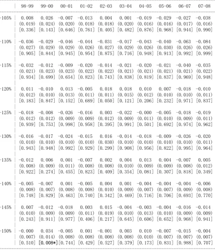
Table 2 presents difference-in-differences estimates of the spillover effects, using those
between 150% of the new minimum wage and the median as the comparison group, 1997-98
as the comparison year, and £3.40 as the lower threshold for the 1997 groups. Modifications
of these specification choices are considered below. The range between 150% of the
minimum and the median is chosen as the comparison group to be as close to the groups
being examined in terms of unobservables as possible. There is a trade-off here. Raising the
comparison group up the distribution reduces the risk that it is itself affected by spillovers, but
reduces the similarity with the groups with which it is being compared.
For each group and each year a block of three statistics is given in the table. The first is the
difference-in-differences estimator of the spillover effect for the specified wage group as a
result of the minimum wage increase in the specified time interval, i.e. the extent to which
wage growth was higher than would have been expected if the minimum wage had not been
raised. For example, looking at the 2001-02 column, i.e. the effect of the October 2001
increase in the minimum wage, the estimate for the first group immediately above the new
minimum (up to 5% above) indicates a negative effect of about 1 percentage point. implying
that wage growth for this group was actually lower than would have been expected in the
absence of the uprating. For this wage group, the estimated effects for the other minimum
wage upratings, from October 2000 to October 2007, are more often negative than positive.
The second statistic in the block, given in parentheses, is the robust standard error of the
difference-in-differences estimate of the spillover effect and the third statistic, given in square
brackets, is the p-value of the test for a positive spillover effect (and hence using a 1-sided
alternative). A p-value less than 0.05, for example, implies that the estimated spillover effect
highlighted in bold. Looking again at the 2001-02 column and the first wage group, the
estimated spillover effect has a standard error of nearly 2 percentage points and hence is
insignificantly different from zero.
Looking at Table 2 as a whole, only 1 out of the 100 estimates is significantly greater than
zero at the 5% significance level. This is less than the rejection rate that one would expect
under the null hypothesis of no positive spillover effects (i.e. the significance level being
used). In addition, the one that is significantly greater than zero is for 1999-2000, which is
viewed, as explained above, as a “no change” year. There are no significantly positive
estimates at all for the minimum wage introduction or any of the upratings for any of the 10
wage groups. There are also more negative estimates in the table than positive ones. The
estimates in the 2001-02 column, i.e. the estimated effects of the October 2001 uprating,
which was the largest in percentage terms and well above the growth in the median, are
negative for all of the first 8 wage groups and insignificant for all 10 wage groups. Overall the
evidence for positive spillover effects from Table 2 is unconvincing.
The results in Table 3 present an equivalent analysis using wage groups similar to those used
by Neumark et al. (2004), stretching far further up the wage distribution. Those with wages
above six times the minimum form the comparison group. Using their groups in the UK
context gives over a quarter of the sample in the group between 2 times and 3 times the
minimum. This group is therefore split in the grouping used here. Only one of the estimates in
Table 3 is significantly greater than zero at the 5% level and this is for 1999-2000, when no
change in the minimum occurred. There are no significant positive effects for the minimum
wage introduction or any of the upratings for any of these wage groups. Once again the
majority of the estimates in Table 3 are negative rather than positive.
A number of robustness checks on these findings were conducted. In all cases the conclusions
drawn from Tables 2 and 3 are confirmed. Tables 2 and 3 give “raw” difference-in-differences
estimates. The equivalent estimates when controls are included for age, sex, part-time,
temporary, company type (7), company size, region (11), and industry (25) are very similar to
those in Tables 2 and 3, and the conclusions are unaltered. For both tables only one estimate
is significantly greater than zero, it is for 1999-2000, viewed as a “no change” year, and it is
Weighting the sample using weights calibrated to the numbers of jobs in a set of calibration
groups in the Labour Force Survey, also does not change the conclusions. For Table 2 there is
only one estimate significantly greater than zero, for 1999-2000 and the same wage group as
before. For Table 3 there are no estimates that are significantly greater than zero.
Tables 2 and 3 use £3.40 as the lower threshold for the first wage group for the reasons
discussed above. The equivalent estimates based on using £3.35 and £3.45 are similar. When
£3.35 is used, for both groupings only one estimate is significantly greater than zero, for
1999-2000 and the same wage group as before. The same is true for the equivalent of Table 3
when £3.45 is used. For the equivalent of Table 2 using £3.45, a second estimate is
significant, but the rejection rate is still below that one would expect under the overall null
hypothesis of no positive spillover effects.
The next modification considered is to the choice of comparison group in Table 2, which uses
the wage range between 50% above the minimum wage and the median wage. The lower limit
is close to the lower quartile point in each year and hence this comparison group covers
roughly 25% of the distribution in each year. (It varies between 20% and 30% over the years.)
Two alternative comparison groups were considered: those between 50% above the minimum
wage and the upper quartile (about 50% of the distribution) and all those more than 50%
above the minimum wage (about 75% of the distribution). In both cases a second estimate is
significant in addition to Table 2, but both again produce rejection rates below what one
would expect under the overall null of no positive spillover effects.
Another alternative considered is to define the groups in terms of constant pence amounts
rather than constant percentage points. A natural one to use has 10 groups of width £0.20. The
comparison group used is the interval between the minimum wage + £2 and the median. This
is slightly wider than that used in Table 2 for earlier years and slightly narrower for later
years. This produces three estimates that are significantly greater than zero, all for the group
between £1.60 and £1.80 above the minimum wage (one of them for 1999-2000). All those
for the first 8 groups are insignificant. Given this insignificance for the nearer groups, these
effects in the 9th group are not credible as spillover effects. Again the rejection rate is still
For the tests conducted so far the samples are restricted to those who remained in the same job
for the 12 month period over which the proportional wage growth is measured. This is the
natural group to investigate. However one might reasonably ask how the results are affected if
this sample restriction is relaxed and estimates conducted on samples containing both those
who remained in the same job and those who moved to a different job. The
difference-in-differences estimates for this wider population are again very similar to those in Tables 2
and 3, and all the main conclusions carry over. For the equivalent of Table 2 only one
estimate is significant and that is for 1999-2000 and the same wage group as before. For the
equivalent of Table 3 there are now no significant estimates.
Overall the evidence from the difference-in-differences estimates does not suggest systematic
spillover effects. The results correspond to what would be expected under the general null
hypothesis of no spillover effects and this conclusion is robust to the various specification
modifications considered, i.e. to modifications to the counterfactual assumed. If anything
there is a lower rejection rate than one would expect under this null. In addition, for all
specifications there are no significant effects for the large October 2001 uprating for any wage
group and no significant effects for any of the first few wage groups above the minimum
wage in any year.
5.2. Estimates using differences between upratings
This section estimates the model that makes use of cross-uprating comparisons. Equation (3)
restricts the variation over time in the spillover effects to be a linear function of the size of the
minimum wage uprating. It still estimates spillover effects separately for each wage group.
Spline terms and control variables are also included. Table 4 gives the results from estimating
equation (3). The left and right halves of the table use the wage groups used in Tables 2 and 3
respectively. Each column of the table represents a separate specification. The specification in
column (1) of each half of the table corresponds to that used in Tables 2 and 3. None of the
estimates, using either specification of the wage groups, is significantly greater than zero. For
the 5% groups specification, the estimates are all negative. For the broader groups
specification, all are negative except that for the top group, which has a p-value of 46%.
As pointed out in section 3, one of the advantages of the approach that makes use of
cross-uprating comparisons, relative to the difference-in-differences approach, is that it does not
require a “no change” period and has less reliance on such a period if one is used. Column (2)
in each half of the table gives the results when the years 1997 and 1998 are not included. This
also removes the need to adopt a particular lower threshold for the first wage group for these
pre-introduction years. Again none of the estimates, using either specification of the wage
groups, is significantly greater than zero, and almost all of them are negative.
As in the previous section, estimates are also given for the case where the sample is expanded
to include those who moved to a different job during the 12 month period over which the
proportional wage growth is measured. Column (3) in each half of the table gives the
estimates when all years are included, while column (4) gives those when 1997 and 1998 are
excluded. Again none of the estimates, using either of these samples and using either
specification of the wage groups, is significantly greater than zero. In column (3) all the
estimates are negative in both cases, while in column (4) all bar one are.
Overall Table 4 does not provide evidence in support of spillover effects. As in the previous
section, a range of robustness checks were conducted. In all cases the conclusions drawn from
Table 4 were confirmed. Estimates were examined using weights calibrated to the Labour
Force Survey; the lower threshold of the first wage group was replaced by £3.35 or £3.45; for
the 5% wage groups specification those between the median and the upper quartile were
added to the base group and then those above the upper quartile were also added; and wage
groups defined in pence rather than percentages were used. In all cases none of the estimates
of any of the wage groups is significantly greater than zero, and almost all of them are
negative. Of the very few positive estimates, the p-values never fall below 21% for the 5%
wage groups and never fall below 35% for the broader wage groups. The evidence for all
these estimates of the specification that makes use of cross-uprating comparisons indicates an
absence of spillover effects. This set of results based on equation (3), similar to that used by
Neumark et al. (2004), therefore paints a very different picture for the impact of the UK
7. Conclusions
This paper investigates possible spillover effects of the UK minimum wage. It uses a very
natural approach to the analysis of spillovers. It asks whether the observed individual wage
changes of those initially (i.e. prior to a particular uprating) in a specified interval above the
new uprated minimum wage are higher than the counterfactual wage changes that one would
expect to observe if the minimum wage had not been raised.
Two econometric approaches are taken in this paper to address this question. The first uses
simple difference-in-differences estimators. The second makes use of cross-uprating
comparison information. The analysis using the difference-in-differences approach does not
find systematic spillovers and the results strongly support an overall null hypothesis of no
spillover effects. The estimates for the models using cross-uprating comparison information
also find no evidence of significant spillovers.
It has been suggested that spillover effects could offer an explanation for the different
behaviour since the mid 1990s of lower tail inequality (as measured by the 50:10 percentile
ratio) and upper tail inequality. However, since the UK minimum wage has always been
below the 10th percentile since its introduction, this absence of spillovers implies that
minimum wage changes have not had an effect on the 50:10 percentile ratio measure of lower
tail wage inequality. The absence of spillovers also importantly offers support for the
identifying assumption in the set of studies of minimum wage effects on various outcomes
References
Autor, D.H., Katz, L. and Kearney, M. (2008), “Trends in U.S. wage inequality: Re-assessing
the revisionists”, Review of Economics and Statistics, 90, 300-23.
Autor, D.H., Manning, A. and Smith, C.L. (2010), “The contribution of the minimum wage
to US wage inequality over three decades: a reassessment”, NBER Working Paper
16533.
Bird, D. (2004), “Methodology for the 2004 Annual Survey of Hours and Earnings”, Labour
Market Trends, November, 457-64.
Butcher, T., Dickens, R. and Manning, A. (2009), “The impact of the NMW on the wage
distribution”, Research for the Low Pay Commission.
Card, D. and Krueger, A.B. (1995), Myth and Measurement: The New Economics of the
Minimum Wage, Princeton University Press.
Dickens, R. and Manning, A. (2004a), “Has the national minimum wage reduced UK wage
inequality?”, Journal of the Royal Statistical Society A, 167, 613-26.
Dickens, R. and .Manning, A. (2004b), “Spikes and spillovers: The impact of the national
minimum wage on the wage distribution in a low wage sector”, Economic Journal, 114, C95-101.
Dickens, R., Riley, R. and Wilkinson, D. (2009), “The Employment and Hours of Work
Effects of the Changing National Minimum Wage”, Report to the Low Pay
Commission.
DiNardo, J., Fortin, N. and Lemieux, T. (1996), “Labor market institutions and the
distribution of wages, 1973-1992: A semiparametric approach”, Econometrica, 64, 1001-44.
Dobbs, C. (2009), “Patterns of pay: results of the Annual Survey of Hours and Earnings, 1997
to 2008”, Economic & Labour Market Review, 3(3), 24-32.
Falk, A., Fehr, E. and Zehnder, C. (2006), “Fairness perceptions and reservation wages - the
behavioural effects of minimum wage laws”, Quarterly Journal of Economics, 121, 1347-81.
Flinn, C.J. (2006), “Minimum wage effects on labour market outcomes under search,
matching, and endogenous contact rates”, Econometrica, 74, 1013-62.
Lee, D. (1999), “Wage inequality in the United States during the 1980s: Rising dispersion or
Low Pay Commission (2009), National Minimum Wage, LPC Report 2009, Cm 7611, The Stationery Office.
Machin, S. (2011), “Changes in UK wage inequality over the last forty years” in Gregg, P.
and Wadsworth, J. (eds), The Labour Market in Winter: The State of Working Britain. Oxford: Oxford University Press.
Manning, A. (2011), “Minimum wages and wage inequality”, in Marsden, D. (ed), Labour
Market Policy for the Twenty-First Century. Oxford: Oxford University Press.
Neumark, D., Schweitzer, M. and Wascher, W. (2004), “Minimum wage effects throughout
the wage distribution”, Journal of Human Resources, 39, 425-50.
Neumark, D. and Wascher, W.L. (2008), Minimum Wages, Cambridge: MIT Press.
Robinson, H. and Wadsworth, J. (2007), “Did the minimum wage affect the incidence of
second job holding in Britain?”, Scottish Journal of Political Economy, 54, 553-74. Stewart, M.B. (2004), “The impact of the introduction of the UK minimum wage on the
employment probabilities of low-wage workers”, Journal of the European Economic
Association, 2, 67-97.
Stewart, M.B. (2011), “Quantile estimates of counterfactual distribution shifts and the impact
of minimum wage increases on the wage distribution”, Warwick Economic Research
Paper 985, forthcoming in Journal of the Royal Statistical Society, Series A.
Stewart, M.B. and Swaffield, J.K. (2008), “The other margin: Do minimum wages cause
working hours adjustments for low-wage workers?”, Economica, 75, 148-67.
Stigler, G.J. (1946), “The economics of minimum wage legislation”, American Economic
Review, 36, 358-65.
Swaffield, J.K. (2008), “How has the minimum wage affected the wage growth of low-wage
Table 1
Average growth rates by wage group
--- | 97-98 98-99 99-00 00-01 01-02 02-03 03-04 04-05 05-06 06-07 07-08 --- Below | 0.541 0.463 0.437 0.231 0.276 0.529 0.251 0.323 0.237 0.178 0.172 -105% | 0.163 0.172 0.189 0.168 0.151 0.172 0.162 0.150 0.129 0.128 0.116 -110% | 0.180 0.146 0.152 0.147 0.137 0.154 0.162 0.144 0.136 0.109 0.088 -115% | 0.143 0.112 0.131 0.146 0.123 0.134 0.119 0.129 0.117 0.095 0.099 -120% | 0.112 0.124 0.102 0.138 0.108 0.135 0.128 0.128 0.115 0.086 0.093 -125% | 0.118 0.102 0.110 0.104 0.104 0.127 0.094 0.124 0.109 0.092 0.091 -130% | 0.117 0.103 0.101 0.105 0.104 0.138 0.101 0.105 0.103 0.083 0.088 -135% | 0.099 0.088 0.105 0.112 0.092 0.106 0.100 0.117 0.098 0.083 0.095 -140% | 0.095 0.091 0.089 0.109 0.091 0.105 0.094 0.097 0.087 0.083 0.081 -145% | 0.099 0.107 0.087 0.093 0.102 0.119 0.093 0.101 0.090 0.074 0.075 -150% | 0.086 0.087 0.120 0.093 0.088 0.090 0.086 0.101 0.074 0.063 0.073 Above | -Med | 0.073 0.074 0.073 0.086 0.074 0.078 0.071 0.079 0.068 0.065 0.064 -UQ | 0.061 0.057 0.063 0.074 0.063 0.060 0.060 0.071 0.056 0.056 0.062
top | 0.040 0.040 0.041 0.068 0.053 0.035 0.036 0.059 0.035 0.049 0.042 ---
Notes:
1. Age 22+, on full adult rate, pay not affected by absence 2. Restricted to those in same job after 12 months. Main jobs only 3. 'Below' group contains those below or equal to the new minimum wage '-Med' group is between minimum x 1.5 and median for year
'-UQ' group is between median and upper quartile for year 'top' group is above upper quartile for year
4. Lower threshold for 1997, 98 set at £3.40
Table 2
Difference-in-differences estimates of minimum wage spillover effects
Wage groups of 5% width in terms of percentages above the minimum wage (Comparison group is those between minimum wage x 1.5 and median)
--- | 98-99 99-00 00-01 01-02 02-03 03-04 04-05 05-06 06-07 07-08 --- -105% | 0.008 0.026 -0.007 -0.013 0.004 0.001 -0.019 -0.029 -0.027 -0.038 | (0.019) (0.024) (0.020) (0.018) (0.018) (0.020) (0.016) (0.016) (0.017) (0.016) | [0.336] [0.143] [0.646] [0.761] [0.405] [0.482] [0.876] [0.968] [0.944] [0.990] |
-110% | -0.036 -0.029 -0.046 -0.044 -0.031 -0.017 -0.043 -0.040 -0.063 -0.084 | (0.027) (0.029) (0.029) (0.026) (0.027) (0.029) (0.026) (0.030) (0.026) (0.026) | [0.905] [0.844] [0.945] [0.954] [0.875] [0.716] [0.948] [0.913] [0.992] [0.999] |
-115% | -0.032 -0.012 -0.009 -0.020 -0.014 -0.021 -0.020 -0.021 -0.040 -0.035 | (0.021) (0.023) (0.023) (0.022) (0.022) (0.021) (0.021) (0.021) (0.021) (0.022) | [0.934] [0.699] [0.654] [0.823] [0.743] [0.838] [0.819] [0.837] [0.969] [0.948] |
-120% | 0.011 -0.010 0.013 -0.005 0.018 0.018 0.010 0.007 -0.018 -0.010 | (0.012) (0.010) (0.013) (0.011) (0.011) (0.015) (0.012) (0.010) (0.010) (0.011) | [0.183] [0.847] [0.152] [0.689] [0.050] [0.121] [0.206] [0.232] [0.971] [0.837] |
-125% | -0.018 -0.008 -0.026 -0.016 0.003 -0.022 -0.000 -0.005 -0.018 -0.019 | (0.012) (0.012) (0.009) (0.009) (0.012) (0.009) (0.011) (0.010) (0.009) (0.011) | [0.939] [0.753] [0.998] [0.958] [0.395] [0.991] [0.501] [0.692] [0.974] [0.962] |
-130% | -0.016 -0.017 -0.024 -0.015 0.016 -0.014 -0.018 -0.009 -0.026 -0.020 | (0.010) (0.010) (0.010) (0.010) (0.030) (0.010) (0.010) (0.010) (0.010) (0.011) | [0.943] [0.948] [0.992] [0.929] [0.299] [0.908] [0.956] [0.822] [0.995] [0.964] |
-135% | -0.012 0.006 0.001 -0.007 0.002 0.004 0.013 0.004 -0.007 0.005 | (0.008) (0.009) (0.011) (0.008) (0.008) (0.010) (0.009) (0.009) (0.008) (0.012) | [0.922] [0.274] [0.455] [0.823] [0.409] [0.354] [0.081] [0.307] [0.818] [0.349] |
-140% | -0.005 -0.007 0.001 -0.005 0.004 0.001 -0.004 -0.004 -0.004 -0.006 | (0.008) (0.007) (0.008) (0.008) (0.010) (0.009) (0.007) (0.007) (0.009) (0.008) | [0.748] [0.829] [0.463] [0.740] [0.342] [0.469] [0.716] [0.706] [0.693] [0.770] |
-145% | 0.007 -0.012 -0.018 0.003 0.015 -0.004 -0.003 -0.004 -0.016 -0.014 | (0.010) (0.009) (0.009) (0.011) (0.019) (0.010) (0.013) (0.010) (0.009) (0.009) | [0.243] [0.911] [0.977] [0.406] [0.217] [0.645] [0.606] [0.652] [0.968] [0.941] |
-150% | -0.000 0.034 -0.005 0.001 -0.001 0.003 0.010 -0.007 -0.015 -0.004 | (0.007) (0.014) (0.008) (0.008) (0.008) (0.008) (0.010) (0.007) (0.007) (0.007) | [0.510] [0.008*][0.744] [0.429] [0.527] [0.379] [0.173] [0.831] [0.988] [0.707] ---
Notes:
Table 3
Difference-in-differences estimates of minimum wage spillover effects Broader wage groups
(Comparison group is those above the minimum wage x 6)
--- | 98-99 99-00 00-01 01-02 02-03 03-04 04-05 05-06 06-07 07-08 --- -110% | -0.017 0.001 -0.059 -0.043 -0.009 -0.001 -0.057 -0.035 -0.076 -0.072 | (0.018) (0.020) (0.020) (0.018) (0.018) (0.019) (0.018) (0.019) (0.018) (0.017) | [0.823] [0.484] [0.998] [0.991] [0.700] [0.513] [0.999] [0.966] [1.000] [1.000] |
-120% | -0.007 -0.005 -0.027 -0.027 0.013 0.009 -0.027 -0.004 -0.056 -0.029 | (0.014) (0.014) (0.016) (0.014) (0.014) (0.015) (0.015) (0.014) (0.014) (0.014) | [0.696] [0.645] [0.954] [0.971] [0.182] [0.272] [0.970] [0.612] [1.000] [0.979] |
-130% | -0.012 -0.006 -0.054 -0.028 0.020 -0.008 -0.032 -0.005 -0.050 -0.026 | (0.010) (0.011) (0.011) (0.010) (0.019) (0.010) (0.011) (0.010) (0.011) (0.011) | [0.884] [0.698] [1.000] [0.997] [0.147] [0.789] [0.998] [0.683] [1.000] [0.992] |
-150% | -0.000 0.008 -0.034 -0.016 0.013 0.010 -0.021 -0.001 -0.040 -0.012 | (0.009) (0.009) (0.010) (0.009) (0.010) (0.009) (0.009) (0.008) (0.010) (0.009) | [0.518] [0.170] [1.000] [0.964] [0.081] [0.113] [0.988] [0.561] [1.000] [0.913] |
-200% | 0.003 0.008 -0.025 -0.011 0.012 0.009 -0.025 0.001 -0.030 -0.007 | (0.008) (0.008) (0.010) (0.008) (0.008) (0.008) (0.008) (0.008) (0.009) (0.009) | [0.336] [0.156] [0.996] [0.914] [0.074] [0.111] [0.999] [0.450] [0.999] [0.790] |
-250% | -0.006 -0.003 -0.037 -0.022 0.000 0.009 -0.028 -0.005 -0.032 -0.007 | (0.008) (0.008) (0.010) (0.008) (0.009) (0.008) (0.008) (0.008) (0.009) (0.009) | [0.766] [0.647] [1.000] [0.995] [0.477] [0.116] [1.000] [0.717] [1.000] [0.781] |
-300% | -0.004 0.007 -0.024 -0.012 0.001 0.007 -0.018 -0.001 -0.028 0.003 | (0.008) (0.008) (0.010) (0.008) (0.008) (0.008) (0.009) (0.008) (0.009) (0.009) | [0.674] [0.175] [0.994] [0.923] [0.455] [0.186] [0.982] [0.569] [0.999] [0.376] |
-400% | -0.001 0.015 -0.023 -0.002 0.003 0.012 -0.015 0.002 -0.018 0.001 | (0.008) (0.008) (0.010) (0.008) (0.008) (0.008) (0.008) (0.009) (0.009) (0.009) | [0.573] [0.040*][0.991] [0.590] [0.350] [0.066] [0.963] [0.387] [0.975] [0.469] |
-500% | 0.006 0.007 -0.008 -0.002 -0.000 0.009 -0.017 0.001 -0.018 0.001 | (0.009) (0.008) (0.010) (0.009) (0.009) (0.008) (0.009) (0.009) (0.010) (0.011) | [0.244] [0.208] [0.788] [0.573] [0.517] [0.148] [0.972] [0.475] [0.971] [0.477] |
-600% | -0.003 0.005 -0.018 0.001 -0.005 -0.000 -0.010 -0.014 0.005 0.001 | (0.010) (0.010) (0.011) (0.011) (0.010) (0.010) (0.011) (0.010) (0.024) (0.011) | [0.640] [0.310] [0.942] [0.448] [0.691] [0.519] [0.808] [0.923] [0.426] [0.455] ---
Notes:
1. Age 22+, on full adult rate, pay not affected by absence. 2. Restricted to those in same job after 12 months. Main jobs only. 3. Robust standard errors in brackets. p-values (1-sided) in square brackets. 4. Comparison group is those above the minimum wage x 6.
Table 4
Spillover estimates using models with size-of-uprating interactions
---
| (1) (2) (3) (4) | | (1) (2) (3) (4) ---
-105% | -0.157 -0.165 -0.204 -0.236 | -110% | -0.250 -0.174 -0.253 -0.182 | (0.124) (0.139) (0.121) (0.136) | | (0.099) (0.101) (0.095) (0.099) | [0.899] [0.881] [0.955] [0.958] | | [0.994] [0.958] [0.996] [0.967]
| | |
-110% | -0.105 0.026 -0.062 0.070 | -120% | -0.246 -0.232 -0.256 -0.240 | (0.123) (0.108) (0.114) (0.104) | | (0.080) (0.080) (0.079) (0.080) | [0.804] [0.405] [0.708] [0.251] | | [0.999] [0.998] [0.999] [0.999]
| | |
-115% | -0.214 -0.151 -0.202 -0.141 | -130% | -0.270 -0.259 -0.304 -0.297 | (0.107) (0.091) (0.104) (0.093) | | (0.072) (0.083) (0.070) (0.081) | [0.977] [0.951] [0.974] [0.935] | | [1.000] [0.999] [1.000] [1.000]
| | |
-120% | -0.024 -0.046 -0.045 -0.078 | -150% | -0.196 -0.199 -0.216 -0.211 | (0.075) (0.082) (0.073) (0.080) | | (0.058) (0.065) (0.057) (0.065) | [0.627] [0.714] [0.733] [0.834] | | [1.000] [0.999] [1.000] [0.999]
| | |
-125% | -0.122 -0.100 -0.192 -0.187 | -200% | -0.160 -0.173 -0.179 -0.188 | (0.068) (0.077) (0.067) (0.076) | | (0.052) (0.057) (0.052) (0.058) | [0.964] [0.903] [0.998] [0.993] | | [0.999] [0.999] [1.000] [0.999]
| | |
-130% | -0.163 -0.141 -0.154 -0.136 | -250% | -0.139 -0.121 -0.135 -0.105 | (0.086) (0.106) (0.081) (0.101) | | (0.052) (0.057) (0.052) (0.057) | [0.971] [0.907] [0.971] [0.912] | | [0.996] [0.983] [0.995] [0.966]
| | |
-135% | -0.087 -0.107 -0.120 -0.114 | -300% | -0.119 -0.120 -0.104 -0.103 | (0.058) (0.067) (0.059) (0.067) | | (0.052) (0.058) (0.053) (0.058) | [0.933] [0.946] [0.979] [0.955] | | [0.988] [0.982] [0.977] [0.961]
| | |
-140% | -0.064 -0.056 -0.077 -0.076 | -400% | -0.066 -0.077 -0.063 -0.065 | (0.051) (0.058) (0.053) (0.059) | | (0.053) (0.060) (0.053) (0.060) | [0.892] [0.835] [0.929] [0.900] | | [0.890] [0.901] [0.881] [0.861]
| | |
-145% | -0.006 0.014 -0.007 -0.002 | -500% | -0.050 -0.066 -0.049 -0.054 | (0.078) (0.090) (0.075) (0.087) | | (0.055) (0.061) (0.055) (0.061) | [0.533] [0.438] [0.539] [0.510] | | [0.816] [0.859] [0.815] [0.813]
| | |
-150% | -0.115 -0.145 -0.111 -0.138 | -600% | 0.007 0.028 -0.001 0.011 | (0.073) (0.091) (0.072) (0.090) | | (0.070) (0.076) (0.069) (0.076) | [0.943] [0.945] [0.937] [0.938] | | [0.462] [0.354] [0.506] [0.444] ---
Notes:
1. Age 22+, on full adult rate, pay not affected by absence.
2. Robust standard errors in brackets. p-values (1-sided) in square brackets. 3. Lower threshold set at £3.40 for pre-introduction (when included). 4. See text for list of control variables included.
5. Samples:
(1) All years, restricted to those in same job after 12 months.
(2) Excluding 1997 & 1998, restricted to those in same job after 12 months. (3) All years, including job changers.
(4) Excluding 1997 & 1998, including job changers. 6. * = estimate significantly greater than zero at the 5% level.