Iterative methods for the force based quasicontinuum approximation : analysis of a 1D model problem

http://wrap.warwick.ac.uk/

Original citation:

Dobson, M., Luskin, M. and Ortner, Christoph. (2011) Iterative methods for the

force-based quasicontinuum approximation : analysis of a 1D model problem. Computer

Methods in Applied Mechanics and Engineering, Volume 200 (Number 37-40). pp.

2697-2709. ISSN 0045-7825

Permanent WRAP url:

http://wrap.warwick.ac.uk/43918

Copyright and reuse:

The Warwick Research Archive Portal (WRAP) makes this work of researchers of the

University of Warwick available open access under the following conditions. Copyright ©

and all moral rights to the version of the paper presented here belong to the individual

author(s) and/or other copyright owners. To the extent reasonable and practicable the

material made available in WRAP has been checked for eligibility before being made

available.

Copies of full items can be used for personal research or study, educational, or

not-for-profit purposes without prior permission or charge. Provided that the authors, title and

full bibliographic details are credited, a hyperlink and/or URL is given for the original

metadata page and the content is not changed in any way.

Publisher’s statement:

NOTICE: this is the author’s version of a work that was accepted for publication in

Computer Methods in Applied Mechanics and Engineering. Changes resulting from the

publishing process, such as peer review, editing, corrections, structural formatting, and

other quality control mechanisms may not be reflected in this document. Changes may

have been made to this work since it was submitted for publication. A definitive version

was subsequently published in Methods in Applied Mechanics and Engineering, (2011)

Volume 200 (Number 37-40). pp. 2697-2709.

http://dx.doi.org/10.1016/j.cma.2010.07.008

note on versions:

The version presented here may differ from the published version or, version of record, if

you wish to cite this item you are advised to consult the publisher’s version. Please see

the ‘permanent WRAP url’ above for details on accessing the published version and note

that access may require a subscription.

Force-based Quasicontinuum Approximation

Matthew Dobson, Mitchell Luskin, and Christoph Ortner

Abstract Force-based multiphysics coupling methods have become popular since they provide a simple and efficient coupling mechanism, avoiding the difficulties in formulating and and implementing a consistent coupling energy. They are also the only known pointwise consistent methods for coupling a general atomistic model to a finite element continuum model. However, the development of efficient and reli-able iterative solution methods for the force-based approximation presents a chal-lenge due to the non-symmetric and indefinite structure of the linearized force-based quasicontinuum approximation, as well as to its unusual stability properties. In this paper, we present rigorous numerical analysis and computational experiments to systematically study the stability and convergence rate for a variety of linear sta-tionary iterative methods.

1 Introduction

Low energy local minima of crystalline atomistic systems are characterized by highly localized defects such as vacancies, interstitials, dislocations, cracks, and grain boundaries separated by large regions where the atoms are slightly deformed from a lattice structure. The goal of atomistic-to-continuum coupling methods [1–4, 15, 16, 22, 26, 28, 32] is to approximate a fully atomistic model by maintaining the accuracy of the atomistic model in small neighbors surrounding the localized

Matthew Dobson

ERMICS - ENPC, 6 et 8 avenue Blaise Pascal, Cit´e Descartes - Champs sur Marne, 77455 Marne la Vall´ee Cedex 2, France e-mail: [email protected]

Mitchell Luskin

School of Mathematics, 206 Church St. SE, University of Minnesota, Minneapolis, MN 55455, USA, e-mail: [email protected]

Christoph Ortner

Mathematical Institute, St. Giles’ 24–29, Oxford OX1 3LB, UK, e-mail: [email protected]

defects and using the efficiency of continuum coarse-grained models in the vast regions that are only mildly deformed from a lattice structure.

Force-based atomistic-to-continuum methods decompose a computational ref-erence lattice into anatomistic regionA and acontinuum regionC, and assigns forces to representative atoms according to the region they are located in. In the quasicontinuum method, the representative atoms are all atoms in the atomistic re-gion and the nodes of a finite element approximation in the continuum rere-gion. The force-based approximation is thus given by [5, 6, 9, 10, 12, 32]

Fqcf j (y):=

(

Fa

j(y) if j∈A,

Fc

j(y) if j∈C,

whereydenotes the positions of the representative atoms which are indexed by j,

Fa

j(y)denotes the atomistic force at representative atom j,andFcj(y)denotes a

continuum force at representative atom j.

The force-based quasicontinuum method (QCF) uses a Cauchy-Born strain en-ergy density for the continuum model to achieve a patch test consistent approx-imation [6, 10, 24]. We recall that a patch test consistent atomistic-to-continuum approximation exactly reproduces the zero net forces of uniformly strained lat-tices [19, 24, 27]. However, the recently discovered unusual stability properties of the linearized force-based quasicontinuum (QCF) approximation, especially its in-definiteness, present a challenge to the development of efficient and reliable iterative methods [12]. Energy-based quasicontinuum approximations have many attractive features such as more reliable solution methods, but practical patch test consistent, energy-based quasicontinuum approximations have yet to be developed for most problems of physical interest, such as three-dimensional problems with many-body interaction potentials [20, 21, 30].

Rather than attempt an analysis of linear stationary methods for the full nonlinear system, in this paper we restrict our focus to the linearization of a one-dimensional model problem about the uniform deformationyF and consider linear stationary methods of the form

P u(n+1)₋u(n)=αr(n), (1)

wherePis a nonsingular preconditioning operator, the damping parameterα>0 is

fixed throughout the iteration (that is, stationary), and the residual is defined as

r(n):=f₋Lqcf_F u(n).

We will see below that our analysis of this simple model problem already allows us to observe many interesting and crucial features of the various methods. For example, we can distinguish which iterative methods converge up to the critical strainF_∗(see (8) for a discussion of the critical strain), and we obtain first results on their convergence rates.

straight-forward generalizations of results from [9–11, 13]. In Section 4, we review the basic properties of linear stationary iterative methods.

In Section 5, we give an analysis of the Richardson Iteration (P=I) and prove a contraction rate of order 1₋O(N−2)in the`εpnorm (discrete Sobolev norms are

defined in Section 2.1), whereNis the size of the atomistic system.

In Section 6, we consider the iterative solution with preconditioner P=Lqcl_F ,

whereLqcl_F is a standard second order elliptic operator, and show that the precon-ditioned iteration with an appropriately chosen damping parameterα is a

contrac-tion up to the critical strainF_∗only inU2,∞_{among the common discrete Sobolev}

spaces. We show, however, that a rate of contraction inU2,∞_{independent ofNcan}

be achieved with the elliptic preconditionerLqcl_F and an appropriate choice of the damping parameterα.

In Section 7, we consider the popular ghost force correction iteration (GFC) which is given by the preconditionerP=Lqce_F ,and we show that the GFC itera-tion ceases to be a contracitera-tion for any norm at strains less than the critical strain. This result and others presented in Section 7 imply that the GFC iteration might not always reliably reproduce the stability of the atomistic system [11]. We did not find that the GFC method predicted an instability at a reduced strain in our benchmark test [18] (see also [24]). To explain this, we note that our 1D analysis in this paper can be considered a good model for cleavage fracture, but not for the slip instabili-ties studied in [18,24]. We are currently attempting to develop a 2D benchmark test for cleavage fracture to study the stability of the GFC method.

2 The QC Approximations and Their Stability

We give a review of the prototype QC approximations and their stability properties in this section. The reader can find more details in [9, 11].

2.1 Function Spaces and Norms

We consider a one-dimensional atomistic chain whose 2N+1 atoms have the ref-erence positionsxj= jε for ε=1/N.The displacement of the boundary atoms

will be constrained, so the space of admissible displacements will be given by the displacement space

U =

u_∈R2N+1:u−N =uN=0 .

We will use various norms on the spaceU which are discrete variants of the usual Sobolev norms that arise naturally in the analysis of elliptic PDEs.

kv_k`p

ε :=

 



ε∑N<sub>`=−N+1</sub>|v`|p 1/p

, 1_≤p<∞,

max<sub>`=−N+</sub>1,...,N|v`|, p=∞,

and we denote byU0,pthe spaceU equipped with the`εpnorm. The inner product

associated with the`2 εnorm is

hv,w_i:=ε

N

∑

`=−N+1

v`w` forv,w∈U.

We will also use_kf_k`p

ε andhf,gito denote the` p

ε-norm and`2ε-inner product for

arbitrary vectors f,gwhich need not belong toU. In particular, we further define theU1,pnorm

kv_kU1,p:=kv0k_`p

ε,

where(v0)`=v<sub>`</sub>0 =ε−1(v`−v`−1),`=−N+1, . . . ,N, and we letU1,pdenote the

spaceU equipped with theU1,pnorm. Similarly, we define the space U2,pand its associatedU2,pnorm, based on the centered second differencev00<sub>`</sub>=ε−2(v`+1−

2v`+v`−1)for`=−N+1, . . . ,N−1.

We have thatv0_∈R2N forv∈U has mean zero∑Nj=−N+1v0j=0.We can thus

obtain from [9, Equation 9] that

max

v∈U

kv0k_`q

ε=1

hu0,v0_{i ≤} max

σ∈R2N kσk_`q

ε

=1

hu0,σi=ku_kU1,p ≤2 max

v∈U

kv0k_`q

ε=1

hu0,v0_i. (2)

We denote the space of linear functionals onU byU∗.Forg_∈U∗,s=0,1,

and 1_≤p_≤∞, we define the negative norms_kg_kU−s,p by

kg_kU−s,p:= sup

v∈U

kvkUs,q=1

hg,v_i,

where 1_≤q_≤∞ satisfies 1_p+1_q =1. We let U−s,p denote the dual space U∗

equipped with theU−s,pnorm.

For a linear mappingA:U1→U2whereUiare vector spaces equipped with the

norms_{k · kUi},we denote the operator norm ofAby

kA_kL(U1,U2):= sup

v∈U,v6=0

kAv_kU2 kv_kU1 .

IfU1=U2, then we use the more concise notation

kA_kU1:=kA_kL(U1,U1).

IfA:U0,2_→U0,2is invertible, then we can define thecondition numberby

WhenAis symmetric and positive definite, we have that

cond(A) =λ_2NA₋₁/λ₁A

where the eigenvalues ofAare 0<λ₁A≤ ··· ≤λ_2NA₋₁.If a linear mappingA:U _→

U is symmetric and positive definite, then we define theA-inner product and A-norm by

hv,w_iA:=hAv,wi, kvk2A=hAv,vi.

The operatorA:U1→U2isoperator stableif the operator normkA−1kL(U2,U1) is finite, and a sequence of operators Aj :U1,j →U2,j is operator stable if the

sequence _k(Aj)−1kL(U2,j,U1,j) is uniformly bounded. A symmetric operator A:

U0,2_→U0,2 _{is called stable if it is positive definite, and this implies operator}

stability. A sequence of positive definite, symmetric operators Aj :U0,2→U0,2

is calledstableif their smallest eigenvaluesλ₁Aj are uniformly bounded away from

zero.

2.2 The atomistic model

We now consider a one-dimensional atomistic chain whose 2N+3 atoms have the reference positionsxj= jε forε=1/N, and interact only with their nearest and next-nearest neighbors.

We denote the deformed positions byyj, j=−N−1, . . . ,N+1; and we

con-strain the boundary atoms and their next-nearest neighbors to match the uniformly deformed state,yF_j =F jε,whereF>0 is a macroscopic strain, that is,

y₋N−1=−F(N+1)ε, y−N=−FNε,

yN=FNε, yN+1=F(N+1)ε.

(3)

We introduced the two additional atoms with indices_±(N+1)so thaty=yF is an equilibrium of the atomistic model. The total energy of a deformationy_∈R2N+3is

now given by

Ea_(y)

−

N

∑

j=−N

εfjyj,

where

Ea_(y)N+1

∑

j=−N

ε φ

y_j−y_j−1

ε

=

N+1

∑

j=−N

ε φ(y0_j) +

N+1

∑

j=−N+1

ε φ(y0_j+y0_j−1). (4)

Here, φ is a scaled two-body interatomic potential (for example, the normalized Lennard-Jones potential,φ(r) =r−12₋2r−6), and fj, j=−N, . . . ,N,are external

unconstrained atoms,

−Fa

j(ya) =fj for j=−N+1, . . . ,N−1,

ya_j=F jε for j=−N−1,−N,N,N+1,

(5)

where the atomistic force (per lattice spacingε) is given by

Fa

j(y):=−

1

ε ∂Ea(y)

∂yj

=1

ε

n

φ0(y0_j+1) +φ0(y0_j+2+y0_j+1) −

φ0(y0_j) +φ0(y0_j+y0_j−1)o

.

(6)

We linearize (6) by lettingu_∈R2N+3,u±N=u±(N+1)=0, be a “small” displace-ment from the uniformly deformed stateyF_j =F jε; that is, we define

uj=yj−yFj for j=−N−1, . . . ,N+1.

We then linearize the atomistic equilibrium equations (5) about the uniformly de-formed stateyFand obtain a linear system for the displacementua,

(La_Fua)j=fj for j=−N+1, . . . ,N−1,

ua_j=0 for j=₋N₋1,₋N,N,N+1,

where(L_Fav)jis given by

(La_Fv)j:=φF00

−vj+1+2vj−vj−1

ε2

+φ_2F00

−vj+2+2vj−vj−2

ε2

.

Here and throughout we define

φ_F00:=φ00(F) and φ_2F00 :=φ00(2F),

whereφis the interatomic potential in (4). We will always assume thatφ_F00>0 and φ_2F00 <0,which holds for typical pair potentials such as the Lennard-Jones potential

under physically realistic deformations.

The stability properties ofLa_Fcan be understood by using a representation derived in [11],

hLa_Fu,u_i=εAF N

∑

`=−N+1

|u0_`|2₋ε3φ_2F00

N

∑

`=−N

|u00_{`|</sub>2=AFku0k2<sub>`}2

ε−ε 2

φ_2F00 ku00k2_`2

ε, (7)

whereAFis thecontinuum elastic modulus

AF=φF00+4φ2F00 .

Proposition 1.Ifφ_2F00 ≤0, then

min

u∈R2N+3\{0}

u_±N=u_±(N+1)=0

hLa_Fu,u_i ku0_k2_`2

ε

=AF−ε2νεφ2F00 ,

where

νε:= min

u∈R2N+3\{0}

u_±N=u_±(N+1)=0

ku00_k2_`2

ε

ku0_k2 `2

ε .

satisfies0<νε≤C for some universal constant C.

2.2.1 The critical strainF_∗

The previous result shows thatLa_F is positive definite, uniformly asN_→∞, if and only ifAF>0. For realistic interaction potentials,LaFis positive definite in a ground

stateF0>0. For simplicity, we assume thatF0=1, and we ask how far the system

can be “stretched” by applying increasing macroscopic strainsF until it loses its stability. In the limit asN_→∞, this happens at thecritical strain F_∗, which is the smallest number larger thanF0, solving the equation

AF_∗=φ00(F_∗) +4φ00(2F_∗) =0. (8)

2.3 The local QC approximation (QCL)

The local quasicontinuum (QCL) approximation uses the Cauchy-Born approxima-tion to approximate the nonlocal atomistic model by a local continuum model [5,23, 26]. For next-nearest neighbor interactions, the Cauchy-Born approximation reads

φ ε−1(y`+1−y`−1)

≈1

2

φ(2y0_{`</sub>) +φ(2y0<sub>`+1})],

and results in the QCL energy, fory_∈R2N+3satisfying the boundary conditions (3),

Eqcl_{(y) =} N

∑

j=−N+1

εφ(y0_j) +φ(2y0_j)

+ε

φ(y0_−N) +1

2φ(2y

0

−N) +φ(y0N+1) +

1 2φ(2y

0

N+1)

.

(9)

−Fqcl j (y

qcl_{) =f}

j for j=−N+1, . . . ,N−1,

yqcl_j =F jε for j=−N,N,

where

Fqcl

j (y):=−

1

ε

∂Eqcl(y)

∂yj

=1

ε

n

φ0(y0_j+1) +2φ0(2y0_j+1) −

φ0(y0_j) +2φ0(2y0_j)o

.

(10)

We see from (10) that the QCL equilibrium equations are well-defined with only a single constraint at each boundary, and we can restrict our consideration to y_∈R2N+1withy−N=−FandyN=Fas the boundary conditions.

Linearizing the QCL equilibrium equations (10) aboutyFresults in the system

(L_Fqcluqcl)j= fj for j=−N+1, . . . ,N−1,

uqcl_j =0 for j=−N,N,

where

Lqcl_F =AFL

andLis the discrete Laplacian, forv_∈U, given by

(Lv)j:=−v00j=

−vj+1+2vj−vj−1

ε2

, j=₋N+1, . . . ,N₋1. (11)

The QCL operator is a scaled discrete Laplace operator, so

hLqcl_F u,u_i=AFku0k2_`2

ε

for allu_∈U.

In particular, it follows thatLqcl_F is stable if and only ifAF>0, that is, if and only if

F<F_∗,whereF_∗is the critical strain defined in (8).

2.4 The force-based QC approximation (QCF)

The force-based quasicontinuum (QCF) method combines the accuracy of the atom-istic model with the efficiency of the QCL approximation by decomposing the com-putational reference lattice into anatomistic regionA and acontinuum regionC, and assigns forces to atoms according to the region they are located in. The QCF operator is given by [5, 6]

Fqcf j (y):=

(

Fa

j(y) if j∈A,

Fqcl

j (y) if j∈C,

and the QCF equilibrium equations are given by

−Fjqcf(y qcf_{) =f}

j for j=−N+1, . . . ,N−1,

yqcf_j =F jε for j=−N,N.

We note that, since atoms near the boundary belong toC, only one boundary con-dition is required at each end.

For simplicity, we specify the atomistic and continuum regions as follows. We fixK_∈N, 1≤K≤N−2, and define

A =_{−K, . . . ,K_} and C =_{−N+1, . . . ,N₋1_{} \}A.

Linearizing (12) aboutyF, we obtain

(Lqcf_F uqcf)j=fj for j=−N+1, . . . ,N−1,

uqcf_j =0 for j=−N,N, (13)

where the linearized force-based operator is given explicitly by

(Lqcf_F v)j:=

(Lqcl_F v)j, for j∈C,

(La_Fv)j, for j∈A.

The stability analysis of the QCF operatorLqcf_F is less straightforward [9, 10]; we will therefore treat it separately and postpone it to Section 3.

2.5 The original energy-based QC approximation (QCE)

The original energy-based quasicontinuum (QCE) method [26] defines an energy functional by assigning atomistic energy contributions in the atomistic region and continuum energy contributions in the continuum region. For our model problem, we obtain

Eqce_{(y) =}

ε

_∑

`∈AE

a

`(y) +ε

∑

c

`(y) fory∈R2N+1,

where

Ec

`(y) = 12 φ(2y0`) +φ(y0`) +φ(y0`+1) +φ(2y0`+1)

, and

Ea

`(y) = 12 φ(y0`−1+y0`) +φ(y0`) +φ(y0`+1) +φ(y0`+1+y0`+2)

.

(Lqce_F uqce)j−gFj =fj for j=−N+1, . . . ,N−1,

uqce_j =0 for j=−N,N, (14)

where, for 0_≤j_≤N₋1,we have

(Lqce_F v)j=φF00−

vj+1+2vj−vj−1

ε2

+φ_2F00

                                  

4−vj+2+2vj−vj−2

4ε2 , 0≤j≤K−2,

4−vj+2+2vj−vj−2 4ε2 +

1

ε

vj+2−vj

2ε , j=K−1,

4−vj+2+2vj−vj−2 4ε2 −

2

ε

vj+1−vj

ε +

1

ε

vj+2−vj

2ε , j=K,

4−vj+1+2vj−vj−1

ε2 −

2

ε

vj−vj−1

ε +

1

ε

vj−vj−2

2ε , j=K+1,

4−vj+1+2vj−vj−1

ε2 +

1

ε

vj−vj−2

2ε , j=K+2,

4−vj+1+2vj−vj−1

ε2 , K+3≤j≤N−1,

and where the vector of “ghost forces,”g, is defined by

gF_j =

                  

0, 0_≤ j_≤K₋2,

−1

2εφ2F0 , j=K−1, 1

2εφ2F0 , j=K, 1

2εφ2F0 , j=K+1,

−1

2εφ2F0 , j=K+2,

0, K+3_≤j_≤N₋1.

The equations for j=₋N+1, . . . ,₋1 follow from symmetry.

The following result is a new sharp stability estimate for the QCE operatorLqce_F . Its somewhat technical proof is given in Appendix 8.1.

Theorem 1.If K_≥1, N_≥K+2, andφ_2F00 ≤0, then

inf

u∈U

ku0k_`2

ε

=1

hLqce_F u,u_i=AF+λKφ_2F00 ,

where 1_2≤λK≤1. Asymptotically, as K→∞, we have

2.6 The quasi-nonlocal QC approximation (QNL)

The QCF method is the simplest idea to circumvent the interface inconsistency of the QCE method, but gives non-conservative equilibrium equations [5]. An alterna-tive energy-based approach was suggested in [14, 33], which is based on a modi-fication of the energy at the interface. The quasi-nonlocal approximation (QNL) is given by the energy functional

Eqnl_(y):=

ε

N

∑

`=−N+1

φ(y0_`) +ε

_∑

`∈A

φ(y0_{`</sub>+y0<sub>`+1}) +ε

_∑

`∈C

1 2

φ(2y0_{`</sub>) +φ(2y0<sub>`+1})

,

where we setφ(y0_−N) =φ(y0_N+1) =0. The QNL approximation is patch test consis-tent; that is,y=yFis an equilibrium of the QNL energy functional.

The linearization of the QNL equilibrium equations aboutyFis

(Lqnl_F uqnl)j=fj for j=−N+1, . . . ,N−1,

uqnl_j =0 for j=−N,N,

where

(Lqnl_F v)j=φF00−

vj+1+2vj−vj−1

ε2

+φ_2F00

          

         

4−vj+2+2vj−vj−2

4ε2 , 0≤j≤K−1,

4−vj+2+2vj−vj−2 4ε2 −

−vj+2+2vj+1−vj

ε2 , j=K,

4−vj+1+2vj−vj−1

ε2 +

−vj+2vj−1−vj−2

ε2 , j=K+1,

4−vj+1+2vj−vj−1

ε2 , K+2≤j≤N−1.

(15)

We can repeat our stability analysis for the periodic QNL operator in [11, Sec. 3.3] verbatim to obtain the following result.

Proposition 2.If K<N₋1, andφ2F≤0, then

inf

u∈U

ku0k_`2

ε

=1

hLqnl_F u,u_i=AF.

Remark 1.Sinceφ_2F00 = (AF−φF00)/4,the linearized operators(φF00)−1LaF,(φF00)−1L qcl F ,

3 Stability and Spectrum of the QCF operator

In this section, we give various properties of the linearized QCF operator, most of which are variants of our results in [9, 10]. We first give a result for the non-coercivity of the QCF operator which lies at the heart of many of the difficulties one encounters in analyzing the QCF method.

Theorem 2 (Theorem 1, [10]).Ifφ_F00>0 andφ_2F00 ∈R\ {0}then, for sufficiently

large N,the operator Lqcf_F isnotpositive-definite. More precisely, there exist N0∈N

and C1≥C2>0such that, for all N≥N0and2≤K≤N/2,

−C1N1/2≤ inf v∈U

kv0k_`2

ε

=1

Lqcf_F v,v_{≤ −}C2N1/2.

The proof of Theorem 2 yields also the following asymptotic result on the oper-ator norm ofLqcf_F . Its proof is a straightforward extension of [10, Lemma 2], which covers the casep=2, and we therefore omit it.

Lemma 1.Letφ_2F00 6=0, then there exists a constant C3>0such that for sufficiently

large N, and for2_≤K_≤N/2,

C−₃1N1/p_≤Lqcf_F

L(U1,p_,U−1,p₎≤C3N1/p.

As a consequence of Theorem 2 and Lemma 1, we analyzed the stability ofLqcf_F in alternative norms. By following the proof of [9, Theorem 3] verbatim (see also [9, Remark 3]), we can obtain the following sharp stability result.

Proposition 3.If AF>0andφ2F00 ≤0, then L qcf

F is invertible with

(Lqcf_F )−1

L(U0,∞_,U2,∞₎≤1/AF.

If AF=0,then LqcfF is singular.

This result shows thatLqcf_F is operator stable up to the critical strainF_∗at which the atomistic model loses its stability as well (cf. Section 2.2).

3.1 Spectral properties of

L

in

U

=

`

L_Fqnl. We first observed this numerically in [9, Section 4.4] for the case of periodic boundary conditions. A proof has since been given in [13, Section 3], which trans-lates verbatim to the case of Dirichlet boundary conditions and yields the following result.

Lemma 2.For all N_≥4, 1_≤K_≤N₋2, we have the identity

Lqcf_F =L−1Lqnl_F L. (16)

In particular, the operator Lqcf_F is diagonalizable and its spectrum is identical to the spectrum of Lqnl_F .

We denote the eigenvalues ofLqnl_F (andLqcf_F ) by

0<λ₁qnl≤...λ_`qnl≤...≤λ_2Nqnl₋₁.

The following lemma gives a lower bound forλ₁qnl,an upper bound forλ_2Nqnl₋₁,and

consequently an upper bound for cond(Lqnl_F ) =λ_2Nqnl₋₁/λ₁qnl.

Lemma 3.If K<N₋1andφ_2F00 ≤0, then

λ₁qnl≥2AF, λ_2Nqnl₋₁≤ AF−4φ2F00

ε−2=φ_F00ε−2, and

cond(Lqnl_F ) =λ

qnl 2N−1

λ₁qnl ≤

φ_F00

2AF

ε−2.

For the analysis of iterative methods, we are also interested in the condition num-ber of a basis of eigenvectors ofLqcf_F asN tends to infinity. Employing Lemma 2, we can writeLqcf_F =L−1ΛqcfLwhereLis the discrete Laplacian operator andΛqcf

is diagonal. The columns of L−1 _{are poorly scaled; however, a simple rescaling}

was found in [13, Thm. 3.3] for periodic boundary conditions. The construction and proof translate again verbatim to the case of Dirichlet boundary conditions and yield the following result (note, in particular, that the main technical step, [13, Lemma 4.6] can be applied directly).

Lemma 4.Let AF>0, then there exists a matrix V of eigenvectors for the

force-based QC operator Lqcf_F such thatcond(V)is bounded above by a constant that is independent of N.

3.2 Spectral properties of

L

in

U

QCF system. The operatorL1/2can be understood as a basis transformation to an orthonormal basis inU1,2. Hence, it will be useful to study the spectral properties ofLqcf_F in that space. The relevant (generalized) eigenvalue problem is

Lqcf_F v=λLv, v_∈U, (17)

which can, equivalently, be written as

L−1Lqcf_F v=λv, v∈U, (18)

or as

L−1/2Lqcf_F L−1/2w=λw, w_∈U, (19)

with the basis transformw=L1/2v, in either case reducing it to a standard eigen-value problem in`2

ε. SinceLandL

1/2_{commute, Lemma 2 immediately yields the}

following result.

Lemma 5.For all N_≥4, 1_≤K_≤N₋2 the operator L−1Lqcf_F is diagonalizable and its spectrum is identical to the spectrum of L−1Lqnl_F .

We gave a proof in [12] of the following lemma, which completely characterizes the spectrum ofL−1Lqnl_F , and thereby also the spectrum ofL−1Lqcf_F . We denote the spectrum ofL−1Lqnl_F (andL−1Lqcf_F ) by_{µqnl_j : j=1, . . . ,2N₋1_}.

Lemma 6.Let K_≤N₋2and AF>0, then the (unordered) spectrum of L−1Lqnl_F

(that is, theU1,2-spectrum) is given by

µqnl_j =

(

AF−4φ_2F00 sin2 _4Kjπ₊₄, j=1, . . . ,2K+1,

AF, j=2K+2, . . . ,2N−1.

In particular, ifφ_2F00 ≤0,then

maxjµqnlj

minjµqnlj

=1₋4φ

00

2F

AF

sin2(2K_4K+₊1₄)π= φF00

AF

+4φ2F00

AF

sin2 π 4K+4

= φF00

AF

+O(K−2).

We conclude this study by stating a result on the condition number of the matrix of eigenvectors for the eigenvalue problem (19). Letting ˜V be an orthogonal matrix of eigenvectors of L−1/2L_FqnlL−1/2and ˜Λ the corresponding diagonal matrix, then Lemma 2 yields

L−1/2Lqcf_F L−1/2= L−1L−1/2Lqnl_F L−1/2L

= (_V˜T_L)−1_˜

Λ(V˜TL).

Lemma 7.If AF >0,then there exists a matrixW of eigenvectors for the precon-e ditioned force-based QC operator L−1/2_Lqcf

F L−1/2, such thatcond(We) =O(N2)as N_→∞.

4 Linear Stationary Iterative Methods

In this section, we investigate linear stationary iterative methods to solve the lin-earized QCF equations (13). These are iterations of the form

P u(n)₋u(n−1)=αr(n−1), (20)

wherePis a nonsingular preconditioner, the step size parameterα>0 is constant (that is, stationary), and the residual is defined as

r(n):=f₋Lqcf_F u(n).

The iteration error

e(n):=uqcf₋u(n) satisfies the recursion

Pe(n)= P₋αLqcf_F e(n−1),

or equivalently,

e(n)= I₋αP−1Lqcf_F e(n−1)=:Ge(n−1), (21)

where the operatorG=I₋αP−1Lqcf_F :U _→U is called theiteration matrix. By iterating (21), we obtain that

e(n)= I₋αP−1Lqcf_F ne(0)=Gne(0). (22)

Before we investigate various preconditioners, we briefly review the classical theory of linear stationary iterative methods [29]. We see from (22) that the iterative method (20) converges for every initial guess u(0)_∈U if and only ifGn_→0 as n_→∞.For a given norm_kv_k, forv_∈U,we can see from (22) that the reduction in the error afterniterations is bounded above by

kGn_k= sup

e(0)_∈U

ke(n)_k ke(0)_k.

It can be shown [29] that the convergence of the iteration for every initial guess u(0)_∈U is equivalent to the conditionρ(G)<1,whereρ(G)is thespectral radius ofG,

ρ(G) =max_{|λi|:λiis an eigenvalue ofG}.

lim

n→∞kG

n

k1/n₌

ρ(G)

for any vector norm onU.However, ifρ(G)<1 andkGk ≥1,the Spectral

Ra-dius Theorem does not give any information about how largenmust be to obtain kGn_{k ≤}1.On the other hand, ifρ(G)<1,then there exists a norm_{k · k}such that kG_k<1, so thatGitself is a contraction [17]. In this case, we have the stronger contraction property that

ke(n)_{k ≤ k}G_kke(n−1)_{k ≤ k}G_kn_ke(0)_k.

In the remainder of this section, we will analyze the norm of the iteration matrix, kG_k,for several preconditionersP,using appropriate norms in each case.

5 The Richardson Iteration (

P

=

I

)

The simplest example of a linear iterative method is the Richardson iteration, where P=I. If follows from Lemma 4 that there exists a similarity transformSsuch that

Lqcf_F =S−1ΛqnlS, (23)

where cond(S)_≤C(whereCis independent ofN), andΛqnlis the diagonal matrix

ofU0,2-eigenvalues(λqnl_j )2N_j=−₁1ofLqcf_F . As an immediate consequence, we obtain the identity

Gid(α) =I−αLqcfF =S− 1 _I

−αΛqnlS,

where yields

kGid(α)k_`2

ε ≤cond(S)kI−αΛ qnl

k`2

ε ≤C_j=1max_,...,2N−1

1₋α λqnl_j . (24)

IfAF>0, then it follows from Proposition 2 thatλjqnl>0 for all j, and hence that

the iteration matrixGid(α):=I−αLqcf_F is a contraction in thek · k_`2

ε norm if and

only if 0<α<α_maxid :=2/λ_2Nqnl₋₁.It follows from Lemma 3 thatα_maxid ≤(2ε2)/φ_F00.

We can minimize the contraction constant for Gid(α) in the kvkST_S norm by

choosingα=α_optid :=2/(λ₁qnl+λ_2Nqnl₋₁),and in this case we obtain from Lemma 3

that

Gid αoptid

_`2

ε ≤C

λ_2Nqnl₋₁−λ₁qnl λ_2Nqnl₋₁+λ₁qnl ≤

C

1₋2AFε

2

φ_F00

.

It thus follows that the contraction constant forGid(α)in thek · k_`2

ε norm is only

5.1 Numerical example for the Richardson Iteration

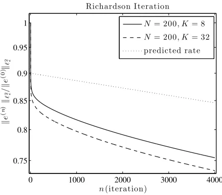
In Figure 1, we plot the error in the Richardson iteration against the iteration number. As a typical example, we use the right-hand side

f(x) =h(x)cos(3πx) where h(x) =

(

1, x_≥0,

−1, x<0, (25)

which is smooth in the continuum region but has a discontinuity in the atomistic region. We choose φ_F00=1,AF =0.5,and the optimal α=α_optid discussed above

(we note thatGid(αoptid)depends only onAF/φF00andN,bute(0)depends onAFand

φ_F00 independently) . We observe initially a much faster convergence rate than the one predicted because the initial residual for (25) has a large component in the eigenspaces corresponding to the intermediate eigenvaluesλ_jqnlfor 1<j<2N₋1.

However, after a few iterations the convergence behavior approximates the predicted rate.

0 1000 2000 3000 4000

0.75 0.8 0.85 0.9 0.95 1

Richardson Iteration

n(iteration)

k

e

(

n

)k

ℓ

2ǫ

/

k

e

(

0

)k

ℓ

2ǫ

N= 200, K= 8 N= 200, K= 32 predicted rate

Fig. 1 Normalized`2

ε-error of successive Richardson iterations for the linear QCF system with

N=200,K=8,32,φ_F00=1,AF=0.5,optimalα=αoptid,right-hand side (25), and starting guess

6 Preconditioning with QCL (

P

=

L

=

A

L

)

We have seen in Section 5 that the Richardson iteration with the trivial precondi-tionerP=Iconverges slowly, and with a contraction rate of the order 1₋O(ε2). The goal of a (quasi-)optimal preconditioner for large systems is to obtain a perfor-mance that is independent of the system size. We will show in the present section that the preconditionerP=AFL(the system matrix for the QCL method) has this

desirable quality.

Of course, preconditioning withP=AFLcomes at the cost of solving a large

linear system at each iteration. However, the QCL operator is a standard elliptic op-erator for which efficient solution methods exist. For example, the preconditioner P=AFLcould be replaced by a small number of multigrid iterations, which would

lead to a solver with optimal complexity. Here, we will ignore these additional com-plications and assume thatPis inverted exactly.

Throughout the present section, the iteration matrix is given by

Gqcl(α):=I−α(LqclF )− 1_Lqcf

F =I−α(AFL)−1LqcfF , (26)

whereα>0 andAF=φF00+4φ2F00 >0. We will investigate whether, ifU is equipped

with a suitable topology,Gqcl(α)becomes a contraction. To demonstrate that this is

a non-trivial question, we first show that in the spacesU1,p, 1_≤p<∞, which are natural choices for elliptic operators, this result does not hold.

Proposition 4.If2_≤K_≤N/2,φ_2F00 6=0,and p∈[1,∞),then for anyα>0we have

Gqcl(α)

_U1,p∼N1/p as N→∞.

Proof. We have from (2) andq=p/(p₋1)the inequality

L−1Lqcf_{F U}1,p = max

u∈U

ku0k_`p

ε= 1

L−1L_Fqcfu 0

_`p

ε

≤ 2 max

u,v∈U

ku0k_`p

ε

=1,kv0k_`q

ε

=1

D

L−1Lqcf_F u0,v0 E

= 2 max

u,v∈U

ku0k_`p

ε= 1,kv0k_`q

ε= 1

D

L L−1Lqcf_F u,vE

= 2 max

u,v∈U

ku0k_`p

ε

=1,kv0k_`q

ε

=1

Lqcf_F u,v

= 2Lqcf_{F L(U}1,p_,U−1,p₎

as well as the reverse inequality

Lqcf_{F L(U}1,p_,U−1,p₎≤

The result now follows from the definition ofGqcl(α)in (26), Lemma 1, and the

fact thatα>0 andAF>0.

We will return to an analysis of the QCL preconditioner in the spaceU1,2 in Section 6.3, but will first attempt to prove convergence results in alternative norms.

6.1 Analysis of the QCL preconditioner in

U

We have found in our previous analyses of the QCF method [9, 10] that it has su-perior properties in the function spacesU1,∞ _andU2,∞_{. Hence, we will now}

in-vestigate whetherα can be chosen such thatGqcl(α)is a contraction, uniformly as

N_→∞. In [9], we have found that the analysis is easiest with the somewhat unusual

choiceU2,∞_{. Hence we begin by analyzingG}

qcl(α)in this space.

To begin, we formulate a lemma in which we compute the operator norm of Gqcl(α)explicitly. Its proof is slightly technical and is therefore postponed to

Ap-pendix 8.2.

Lemma 8.If N_≥4, then

Gqcl(α)_U2,∞=

1−α 1−

2φ₂00_F AF

+α

2φ₂00_F AF

.

What is remarkable (though not necessarily surprising) about this result is that the operator norm ofGqcl(α)is independent ofNandK. This immediately puts us

into a position where we can obtain contraction properties of the iteration matrix Gqcl(α), that are uniform in NandK. It is worth noting, though, that the optimal contraction rate is not uniform asAF approaches zero; that is, the preconditioner

does not give uniform efficiency as the system approaches its stability limit.

Theorem 3.Suppose that N_≥4, AF>0,andφ2F00 ≤0, and define

α_optqcl,2,∞:= AF

AF+2|φ2F00 |

= 2AF

φ_F00+AF

and α_maxqcl,2,∞:=2AF

φ_F00 .

Then Gqcl(α)is a contraction ofU2,∞if and only if0<α<αmaxqcl,2,∞, and for any

such choice the contraction rate is independent of N and K. The optimal choice is

α=α_optqcl,2,∞, which gives the contraction rate

Gqcl αoptqcl,2,∞

_U2,∞=

1−AF_φ00

F

1+AF

φ_F00 <1.

Proof. Note thatαoptqcl,2,∞=1/ 1− 2φ₂00_F

AF

kGqcl(α)k_U2,∞ =1−α 1−2

φ₂00_F AF

−2αφ

00

2F

AF =1−α=:m1(α).

The optimal choice is clearlyα=α_optqcl,2,∞which gives the contraction rate

Gqcl αoptqcl,2,∞

_U2,∞=α

qcl,2,∞

opt

2φ_2F00

AF

=

2_|φ_2F00 | φ_F00+2φ_2F00 =

1−AF_φ00

F

1+AF

φ_F00 .

Alternatively, ifα≥αoptqcl,2,∞,then

Gqcl(α)_U2,∞=α 1−

4φ₂00_F AF

−1=αφ 00

F

AF−

1=:m2(α).

This value is strictly increasing with α, hence the optimal choice is again α =

αoptqcl,2,∞.

Moreover, we havem2(α)<1 if and only if

α<2AF φ_F00 =α

qcl,2,∞

max .

Since, for α =α_optqcl,2,∞ we have m1(α) =m2(α)<1, it follows that αmaxqcl,2,∞>

α_optqcl,2,∞(as a matter of fact, the conditionαmaxqcl,2,∞>α_optqcl,2,∞is equivalent toAF>0).

In conclusion, we have shown that_kGqcl(α)k_U2,∞ is independent ofNandKand

that it is strictly less than one if and only if α <αmaxqcl,2,∞, with optimal value

α=α_optqcl,2,∞.

As an immediate corollary, we obtain the following general convergence result.

Corollary 1.Suppose that N_≥4, AF>0,φ2F00 ≤0, and suppose thatk·kXis a norm

defined onU such that

ku_kX≤CkukU2,∞ ∀u∈U.

Moreover, suppose that0<α<αmaxqcl,2,∞. Then, for any u∈U,

Gqcl(α)nu

X≤qˆ n_C

ku_kU2,∞→0 as n→∞,

whereqˆ:=kGqcl(α)k_U2,∞<1.

In particular, the convergence is uniform among all N, K and all possible initial values u_∈U for which a uniform bound on_ku_kU2,∞ holds.

Proof. We simply note that, according to Theorem 3, for 0<α<αmaxqcl,2,∞, we have

Gqcl(α)n_U2,∞≤qˆ

n_,

where ˆq:=kGqcl(α)k_U2,∞<1 is a number that is independent ofNandK. Hence,

Gqcl(α)nu

X≤C

Gqcl(α)nu

_U2,∞≤Cqˆ

n

ku_kU2,∞.

Remark 2.Although we have seen in Theorem 3 and Corollary 1 that the linear stationary method with preconditionerAFLand with sufficiently small step sizeα

is convergent, this convergence may still be quite slow if the initial data is “rough.” Particularly in the context of defects, we may, for example, be interested in the convergence properties of this iteration when the initial residual is small or moderate inU1,p_{, for somep∈[1,∞], but possibly of orderO(N)in theU}2,∞_{-norm. We can}

see from the following Poincar´e and inverse inequalities

ku_kU1,∞≤

1

2kukU2,∞ and kukU2,∞≤2NkukU1,∞ for allu∈U;

that the application of Corollary 1 to the caseX=U1,∞_{gives the estimate}

Gqcl(α)nu_U1,∞ ≤qˆ

n_N

ku_kU1,∞ for allu∈U.

Similarly, withX=U1,2_{, we obtain}

Gqcl(α)nu_U1,2≤qˆnN3/2kukU1,2 for allu∈U. (27)

We have seen in Proposition 4 that a direct convergence analysis inU1,p_,p<∞,

may be difficult with analytical methods, hence we focus in the next section on the caseU1,∞_.

6.2 Analysis of the QCL preconditioner in

U

As before, we first compute the operator norm of the iteration matrix explicitly. The proof of the following lemma is again postponed to the Appendix 8.2.

Lemma 9.If K_≥3,N_≥max(9,K+3), andφ_2F00 ≤0, then

Gqcl(α)

_U1,∞=

 



1₋α+α4

φ₂00_F AF

for0≤α≤α

qcl,1,∞

opt ,

1₋α 1−2φ 00

2F

AF

+α(6+2ε−4εK)

φ₂00_F AF

forα

qcl,1,∞

opt ≤α,

where

αoptqcl,1,∞:=

h

1+ (2+ε−2εK)

φ₂00_F AF

i−1

satisfiesαoptqcl,2,∞≤α qcl,1,∞

opt ≤1.

Again we note that the operator norm is independent, but now up to terms of order O(εK), of the system size.

Theorem 4.Suppose that K_≥3,N_≥max(9,K+3), andφ_2F00 <0, then the

(i) Ifφ_F00+8φ_2F00 ≤0,then Gqcl(α)isnota contraction ofU1,∞, for any value ofα.

(ii) Ifφ_F00+8φ_2F00 >0,then Gqcl(α)is a contraction for sufficiently smallα. More

precisely, setting

α_maxqcl,1,∞:= 2AF

AF+ (8+2ε−4εK)_|φ_2F00 |,

we have that Gqcl(α)is a contraction ofU1,∞if and only if0<α<αmaxqcl,1,∞. The

operator norm_kGqcl(α)k_U1,∞is minimized by choosingα=α

qcl,1,∞

opt (cf. Lemma

9) and in this case

Gqcl αoptqcl,1,∞

_U1,∞=1−

φ_F00+8φ_2F00

φ_F00+ (2−ε+2εK)φ_2F00 <1.

Proof. Suppose, first, that 0<α≤α_optqcl,1,∞. Sinceα_optqcl,1,∞≤1 it follows that

Gqcl(α)_U1,∞=1−α

φ_F00+8φ_2F00

AF

,

and hence_kGqcl(α)kU1,∞<1 if and only ifφ_F00+8φ_2F00 >0. In that casekGqcl(α)kU1,∞

is strictly decreasing in(0,αoptqcl,1,∞].

Sinceαoptqcl,1,∞≥α qcl,2,∞

opt = (1−2

φ₂00_F AF )

−1_{we can see that}

kGqcl(α)k_U1,∞is always

strictly increasing in[α_optqcl,1,∞,+∞)and hence ifφ_F00+8φ_2F00 >0, thenα =α_optqcl,1,∞

minimizes the operator norm _kGqcl(α)kU1,∞. Moreover, straightforward

compu-tations show that αmaxqcl,1,∞ >αoptqcl,1,∞ and that kGqcl(α)k_U1,∞ <1 if and only if

0<α<αmaxqcl,1,∞.

We remark that the optimal value ofα inU1,∞, that isα =αoptqcl,1,∞, is not the

same as the optimal value,α_optqcl,2,∞,inU2,∞_{. However, it is easy to see thatα}qcl,1,∞

opt =

α_optqcl,2,∞+O(εK), and hence, even thoughα_optqcl,2,∞is not optimal inU1,∞it is still

close to the optimal value. On the other hand,αmaxqcl,1,∞ andαmaxqcl,2,∞are not close,

since, if 4εK−2ε<1,then

α_maxqcl,1,∞≤ 2AF φ_F00+3_|φ_2F00 |<

2AF

φ_F00 =α

qcl,2,∞

max .

In summary, we have seen that the contraction property ofGqcl(α)inU1,∞ is

significantly more complicated than in U2,∞_{, and that, in fact, G}

qcl(α) is not a

6.3 Analysis of the QCL preconditioner in

U

Even though we were able to prove uniform contraction properties for the QCL-preconditioned iterative method inU2,∞_{, we have argued above that these are not}

entirely satisfactory in the presence of irregular solutions containing defects. Hence we analyzed the iteration matrixGqcl(α) =I−α(AFL)−1LFqcfinU1,∞, but there we

showed that it is not a contraction up to the critical loadF_∗. To conclude our results for the QCL preconditioner, we present a discussion ofGqcl(α)in the spaceU1,2.

We begin by noting that it follows from (21) that

P1/2e(n)= P1/2Gqcl(α)e(n−1)=P1/2

I₋αP−1Lqcf_F

P−1/2

P1/2e(n−1)

= I₋αP−1/2Lqcf_F P−1/2 P1/2e(n−1)

=:Geqcl(α)

P1/2e(n−1).

Since_kP1/2v_k`2

ε =A 1/2

F kvkU1,2forv∈U, it follows thatGqcl(α)is a contraction in

U1,2_{if and only if}

e

Gqcl(α)is a contraction in`2ε. Unfortunately, we have shown in

Proposition 4 that_kGqcl(α)kU1,2 ∼N1/2asN→∞. Hence, we will follow the idea used in Section 5 and try to find an alternative norm with respect to whichGe_qcl(α) is a contraction.

From Lemma 5 we deduce that there exists a similarity transform ˜S such that cond(_S˜_)≤N2_{, and such that}

L−1/2Lqcf_F L−1/2=_S˜−1

e

ΛqnlS˜,

whereΛeqnl is the diagonal matrix ofU1,2-eigenvalues(µqnl_j )2N_j=−₁1 ofLqnl_F . As an immediate consequence we obtain

e

Gqcl(α) =S˜−1 I−_Aα

FΛe

qnl_˜ S.

Proceeding as in Section 5, we would obtain that_kGeqcl(α)k_`2

ε ≤O(N

2_{). Instead, we}

observe that

Gqcl(α)u_˜

ST_S˜=

S˜Geqcl(α)u_`2

ε =

(I−_Aα

FΛe

qnl_{)Su˜ `}2

ε

≤ I₋ α

AFΛe

qnl _`2

εk

˜ Su_k`2

ε=_j=1max_,...,2N−1

1₋ α

AFµ

qnl j

kuk_S˜T_S˜,

that is,

eGqcl(α)(α)_˜

ST_S˜≤ max j=1,...,2N−1

1₋ α

AFµ

qnl j

. (28)

Thus, we can conclude thatGeqcl(α)is a contraction in thek · k_S˜T_S˜-norm if and only

if 0<α<αmaxqcl,1,2:=2AF/µ2Nqnl−1. Moreover, we obtain the error bound

where ˜q:= eG_qcl(α) _˜

STS˜. This is slightly worse in fact, than (27), however, we note

that this large prefactor cannot be seen in the following numerical experiment. Moreover, optimizing the contraction rate with respect toα leads to the choice

α_optqcl,1,2:=2AF/(µ₁qnl+µ_2Nqnl₋₁), and in this case we obtain from Lemma 6 that

˜

q=q˜opt:=

eGqcl α_optqcl,1,2_˜

ST_S˜=

µ_2Nqnl₋₁−µ₁qnl µ_2Nqnl₋₁+µ₁qnl ≤

1₋AF

φ_F00

1+AF

φ_F00

,

where the upper bound is sharp in the limit K_→∞. It is particularly interesting

to note that the contraction rate obtained here is precisely the same as the one in

U2,∞_{(cf. Theorem 3). Moreover, it can be easily seen from Lemma 6 thatα}qcl,1,2

opt →

α_optqcl,2,∞asK_→∞, which is the optimal stepsize according to Theorem 3. We further

have thatαmaxqcl,1,2→αmaxqcl,2,∞asK→∞.

6.4 Numerical example for QCL-preconditioning

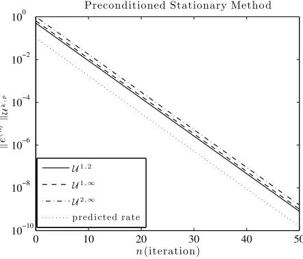
We now apply the QCL-preconditioned stationary iterative method to the QCF sys-tem with right-hand side (25),φ_F00=1,AF=0.2, and the optimal valueα=αoptqcl,2,∞

(we note thatGid(α_optqcl,2,∞)depends only onAF/φF00andN,bute(0)depends onAF

andφ_F00 independently). The error for successive iterations in theU1,2,U1,∞ _and

U2,∞_{-norms are displayed in Figure 2. Even though our theory, in this case, predicts}

a perfect contractive behavior only inU2,∞_{and (partially) in}U1,2_{, we nevertheless}

observe perfect agreement with the optimal predicted rate also in theU1,∞_-norms.

As a matter of fact, the parameters are chosen so that case (i) of Theorem 4 holds, that is,Gqcl(α)isnota contraction ofU1,∞. A possible explanation why we still

observe this perfect asymptotic behavior is that the norm ofGqcl(α)is attained in a

subspace that is never entered in this iterative process. This is also supported by the fact that the exact solution is uniformly bounded inU2,∞_asN,K

→∞, which is a

simple consequence of Proposition 3.

7 Preconditioning with QCE (

P

=

L

): Ghost-Force Correction

We have shown in [5, 12] that the popularghost force correction method (GFC)is equivalent to preconditioning the QCF equilibrium equations by the QCE equilib-rium equations. The ghost force correction method in a quasi-static loading can thus be reduced to the question whether the iteration matrix

0 10 20 30 40 50 10−10

10−8 10−6 10−4 10−2 100

Preconditioned Stationary Metho d

n(iteration)

k

e

(

n

)k

U

k

,

p

U1,2

U1,∞ U2,∞

p red i cted rate

Fig. 2 Error of the QCL-preconditioned linear stationary iterative method for the QCF system with N=800,K=32,φF00=1,AF=0.2, optimal valueα=αoptqcl,2,∞,and right-hand side (25). In this case, the iteration matrixGqcl(α)isnota contraction ofU1,∞_{. Even though our theory predicts a}

perfect contractive behavior only inU2,∞_{, we observe perfect agreement with the optimal predicted}

rate also in theU1,2andU1,∞_-norms.

is a contraction. Due to the typical usage of the preconditionerLqce_F in this case, we do not consider a step sizeαin this section. The purpose of the present section is (i)

to investigate whether there exist function spaces in whichGqceis a contraction; and

(ii) to identify the range of the macroscopic strainsFwhereGqceis a contraction.

We begin by recalling the fundamental stability result for theLqce_F operator, The-orem 1:

inf

u∈U

ku0k_`2

ε

=1

hLqce_F u,u_i=AF+λKφ2F00 ,

whereλK∼λ_∗+O(e−cK)withλ_∗≈0.6595. This result shows that the GFC iteration

must necessarily run into instabilities before the deformation reaches the critical strainF_c∗. This is made precise in the following corollary which states that there is no norm with respect to whichGqceis a contraction up to the critical strainF∗.

Corollary 2.Fix N and K, and let_k·kXbe an arbitrary norm on the spaceU, then,

upon understanding Gqceas dependent onφ_F00andφ_2F00 , we have

kGqcekX→+∞ as AF+λKφ_2F00 →0.

interested in the behavior asN_→∞, that is, we will investigate in which function spaces the operator norm ofGqceremains bounded away from one asN→∞.

The-orem 2 on the unboundedness ofLqcf_F immediately provides us with the following negative answer.

Proposition 5.If2_≤K_≤N/2,φ_2F00 6=0, and AF+λKφ2F00 >0, then

kGqcek_U1,2∼N1/2 as N→∞.

Proof. It is an easy exercise to show that, ifAF+λKφ2F00 >0, then theU1,2-norm is

equivalent to the norm induced byLqce_F , that is,

C−1_ku_kU1,2≤ kuk_Lqce

F ≤CkukU1,2.

Hence, we have_kGqcek_U1,2 ≈ kGqcek_Lqce

F and by the same argument as in the proof

of Proposition 4, and using again the uniform norm-equivalence, we can deduce that

Gqce

_U1,2 ≈

Lqcf_F

L(U1,2_,U−1,2₎±1∼N1/2 asN→∞.

Since the operator(Lqce_F )−1_Lqcf

F is more complicated than that of(AFL)−1LqcfF ,

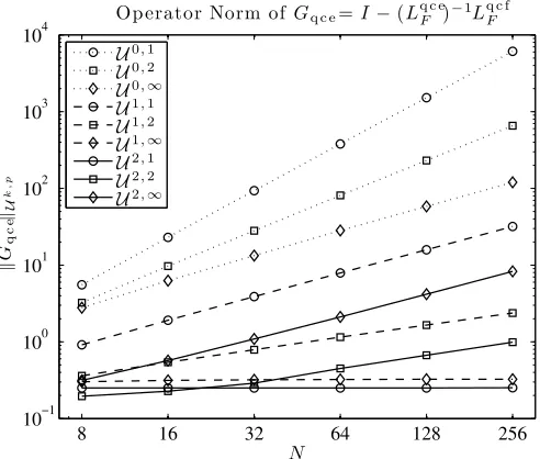
which we analyzed in the previous section, we continue to investigate the contrac-tion properties ofGqcein various different norms in numerical experiments. In

Fig-ure 3, we plot the operator norm ofGqce, in the function spaces

Uk,p_{, k=0,1,2, p=1,2,} ∞,

against the system sizeN (see Appendix 8.3 for a description of how we compute kGqcek_Uk,p). This experiment is performed forAF/φF00=0.8 which is at some

dis-tance from the singularity ofLqce_F (we note thatGqce depends only onAF/φF00 and

N since both(φ_F00)−1Lqcf_F and(φ_F00)−1Lqce_F depend only onAF/φF00 andN). The

ex-periments suggests clearly that_kGqcek_Uk,p→∞asN→∞for all norms except for

U1,∞_andU2,1_.

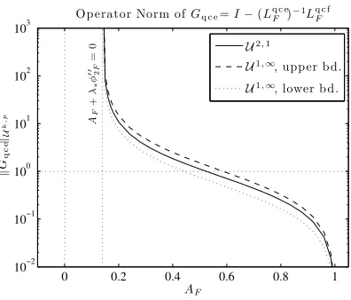
Hence, in a second experiment, we investigate how_kGqcek_U1,∞ andkGqcek_U2,1 behave, for fixedNandK, asAF+λKφ2F00 approaches zero. The results of this

ex-periment, which are are displayed in Figure 4, confirm the prediction of Corol-lary 2 that_kGqcek_Uk,p→∞asAF+λKφ_2F00 approaches zero. Indeed, they show that

kGqcek_Uk,p >1 already much earlier, namely around a strainF whereAF≈0.52

andAF+λKφ_2F00 ≈0.44.

8 16 32 64 128 256 10−1

100 101 102 103 104

N

k

Gq

c

e

kU

k

,

p

Operator Norm of Gq c e=I−(Lq c eF )−1L

q c f F

U0,1

U0,2

U0,∞

U1,1

U1,2

U1,∞

U2,1

U2,2

U2,∞

Fig. 3 Graphs of the operator norm_kGqcek_Uk,p,k=0,1,2,p=1,2,∞, plotted against the number of atoms,N, with atomistic region sizeK=d√N_e−1, andAF/φ_F00=0.8. (The graph for theU1,p

-norms,p=1,∞, are only estimates up to a factor of 1/2; cf. Appendix 8.3.) The graphs clearly indicate that_kGqcek_Uk,p→∞asN_→∞in all spaces except forU1,∞_andU2,1_.

definite statement, it shows at the very least that further investigations for more realistic model problems are required.

Conclusion

We proposed and studied linear stationary iterative solution methods for the QCF method with the goal of identifying iterative schemes that are efficient and reliable for all applied loads. We showed that, if the local QC operator is taken as the pre-conditioner, then the iteration is guaranteed to converge to the solution of the QCF system, up to the critical strain. What is interesting is that the choice of function space plays a crucial role in the efficiency of the iterative method. InU2,∞_{, the}

con-vergence is always uniform inN andK, however, inU1,∞_{this is only true if the}

macroscopic strain is at some distance from the critical strain. This indicates that, in the presence of defects (that is, non-smooth solutions), the efficiency of a QCL-preconditioned method may be reduced. Further investigations for more realistic model problems are required to shed light on this issue.

strains that are far lower than the critical strainF_∗,we show that_kGqcekU1,2∼N1/2. We then give numerical experiments that suggest that_kGqcek_Uk,p →∞asN→∞

for all tested norms except forU1,∞_andU2,1_.

The results presented in this paper demonstrate the challenge for the development of reliable and efficient iterative methods for force-based approximation methods. Further analysis and numerical experiments for two and three dimensional prob-lems are needed to more fully assess the implications of the results in this paper for realistic materials applications.

8 Appendix

8.1 Proof of Theorem 1

The purpose of this appendix is to prove the sharp stability result for the operator L_Fqce, formulated in Theorem 1. Using Formula (23) in [11] we obtain the following representation ofLqce_F ,

0 0.2 0.4 0.6 0.8 1

10−2

10−1

100

101

102

103

AF

k

Gq

c

e

kU

k

,

p

Operator Norm ofGq c e=I−(Lq c eF )−1L

q c f

F

AF

+

λ∗

φ

′′ 2F

=

0 _U2,1

U1,∞_{, upper bd.} U1,∞_{, lower bd.}

Fig. 4 Graphs of the operator norm_kGqcek_Uk,p,(k,p)∈ {(1,∞),(2,1)}, for fixedN=256,K= 15,φ_F00=1, plotted againstAF. For the caseU1,∞only estimates are available and upper and lower

bounds are shown instead (cf. Appendix 8.3). The graphs confirm the result of Corollary 2 that

kGqcek_Uk,p→∞asAF+λKφ₂00_F→0. Moreover, they clearly indicate that_kGqcek_Uk,p>1 already for strainsFin the regionAF≈0.5, which are much lower than the critical strain at whichLqceF

Lqce_F u,u=

(

−K−2

∑

`=−N+1

εAF|u0`|2+

N

∑

`=K+3

εAF|u0`|2 )

+

(

K−1

∑

`=−K+2

ε

AF|u0`|2−ε2φ2F00 |u00`|2

)

+ε

n

(AF−φ2F00 )(|u−0 K+1|2+|u0K|2) +AF(|u0₋K|2+|u0K+1|2)

+ (AF+φ_2F00 )(|u0_−K−1|2+|u0_K+2|2)

−1 2ε

2

φ_2F00 (|u00_−K|2+|u00_−K−1|2+|u00_K|2+|u00_K+1|2)o.

(29)

Ifφ_2F00 <0,then we can see from this decomposition that there is a loss of stability

at the interaction between atoms₋K₋2 and₋K₋1 as well as between atomsK+1 andK+2. It is therefore natural to test this expression with a displacement ˆudefined by

ˆ u0_`=

  

 

1, `=₋K₋1,

−1, `=K+2,

0, otherwise.

From (29), we easily obtain

Lqce_F uˆ,uˆ

=AF+1₂φ2F00 .

In particular, we see that, ifAF+1₂φ_2F00 <0,thenLqce_F is indefinite. On the other

hand, it was shown in [8] thatLqce_F is positive definite providedAF+φ_2F00 >0. (As a

matter of fact, the analysis in [8] is for periodic boundary conditions, however, since the Dirichlet displacement space is contained in the periodic displacement space the result is also valid for the present case.)

Thus, we have shown that

inf

u∈U

ku0k_`2

ε

=1

Lqce_F u,u=AF+µ φ2F00 , where12≤µ≤1.

To conclude the proof of Theorem 1, we need to show thatµdepends only onKand

that the stated asymptotic result holds.

From (29) it follows thatLqce_F can be written in the form

Lqce_F u,u= (u0)THu0,

where we identifyu0 with the vector u0= (u0_`)N

`=−N+1 and whereH ∈R 2N×2N_.

H2=              . ._. . ._. . ._. 1 2 1

1 2 1 1 3/2 1/2

1/2 3 1/2 1/2 9/2 0

0 4 0 0 4 0

. ._. . ._. . ._.             

Here, the row with entries[1,3/2,1/2]denotes theKth row (in the coordinatesu0_k). This form can be verified, for example, by appealing to (29). Letσ(A)denote the spectrum of a matrixA. Since, by assumption,φ_2F00 ≤0, the smallest eigenvalue of

H is given by

minσ(H) =φ_F00+φ_2F00 maxσ(H2),

that is, we need to compute the largest eigenvalue ¯λ ofH2. SinceH2ek=4ekfor

k=K+3,K+4, . . . and forK=₋K₋2,₋K₋3, . . ., and since eigenvectors are orthogonal, we conclude that all other eigenvectors depend only on the submatrix describing the atomistic region and the interface. In particular, ¯λdepends only onK

but not onN. This proves the claim of Theorem 1 thatλK depends indeed only on

K.

We thus consider the_{−K₋1, . . . ,K+2_}-submatrixH¯2, which has the form

¯

H2=

           

9/2 1/2 1/2 3 1/2

1/2 3/2 1

1 2 1

. ._. . ._. . ._.

1 2 1

1 3/2 1/2 1/2 3 1/2

1/2 9/2

            .

LettingH¯2ψ=λ ψ, then for`=−K+2, . . . ,K₋1,

ψ`−1+2ψ`+ψ`+1=λ ψ`,

and hence,ψhas the general form

ψ`=az`+bz−`, `=−K+1, . . . ,K,

leavingψ`undefined for`∈ {−K,−K−1,K+1,K+2}for now, and wherez,1/z are the two roots of the polynomial

z2+ (2₋λ)z+1=0.

z= (1

2λ−1) +

q

(1

2λ−1)2−1>1. (30)

To determine the remaining degrees of freedom, we could now insert this general form into the eigenvalue equation and attempt to solve the resulting problem. This leads to a complicated system which we will try to simplify.

We first note that, for any eigenvectorψ, the vector(ψK−`)is also an eigenvector, and hence we can assume without loss of generality thatψis skew-symmetric about

`=1/2. This implies thata=<sub>−</sub>b. Since the scaling is irrelevant for the eigenvalue problem, we therefore make theansatzψ`=z`−z−`. Next, we notice that forK suf-ficiently large the termz−`is exponentially small and therefore does not contribute to the eigenvalue equation near the right interface. We may safely ignore it if we are only interested in the asymptotics of the eigenvalue ¯λ asK→∞. Thus, letting

ˆ

ψ`=z`,`=1, . . . ,Kand ˆψ`unknown,`=K+1,K+2, we obtain the system

zK−1+3 2z

K₊1

2ψˆK+1= λˆz K_,

1 2z

K_{+3 ˆ}

ψK+1+1₂ψˆK+2= λˆψˆK+1, 1

2ψˆK+1+9₂ψˆK+2= λˆψˆK+2.

The free parameters ˆψK+1,ψˆK+2can be easily determined from the first two

equa-tions. From the final equation we can then compute ˆλ. Upon recalling from (30) that

ˆ

zcan be expressed in terms of ˆλ, and conversely that ˆλ= (zˆ2+1)/zˆ+2, we obtain

a polynomial equation of degree five for ˆz,

q(zˆ):=4ˆz5₋12ˆz4+9ˆz3₋3ˆz2₋4ˆz+2=0.

Mathematica was unable to factorizeqsymbolically, hence we computed its roots numerically to twenty digits precision. It turns out thatqhas three real roots and two complex roots. The largest real root is at ˆz_≈2.206272296 which gives the value

ˆ

λ=zˆ

2₊₁

ˆ

z +2≈4.659525505897.

The relative errors that we had previously neglected are in fact of order ˆz−2K, and hence we obtain

λK=λ_∗+O(e−cK), where λ_∗≈0.6595 and c≈1.5826.

This concludes the proof of Theorem 1.

8.2 Proofs of Lemmas 8 and 9