SDSS J0926+3624 : the shortest period eclipsing binary star

University of Warwick institutional repository: http://go.warwick.ac.uk/wrap

This paper is made available online in accordance with

publisher policies. Please scroll down to view the document

itself. Please refer to the repository record for this item and our

policy information available from the repository home page for

further information.

To see the final version of this paper please visit the publisher’s website.

Access to the published version may require a subscription.

Author(s): C. M. Copperwheat, T. R. Marsh, S. P. Littlefair, V. S.

Dhillon, G. Ramsay, A. J. Drake, B. T. Gänsicke, P. J. Groot, P.

Hakala, D. Koester, G. Nelemans, G. Roelofs, J. Southworth, D.

Steeghs, S. Tulloch

Article: SDSS J0926+3624: the shortest period eclipsing binary star

Year of publication: 2010

Link to published article:

http://link.aps.org/doi/10.1111/j.1365-2966.2010.17508.x

Publisher statement: ‘The definitive version is

arXiv:1008.1907v2 [astro-ph.SR] 13 Aug 2010

SDSS J0926+3624: The shortest period eclipsing binary

star

C.M. Copperwheat

, T.R. Marsh

, S.P. Littlefair

, V.S. Dhillon

, G. Ramsay

,

A.J. Drake

, B.T. G¨

ansicke

, P.J. Groot

, P. Hakala

, D. Koester

, G. Nelemans

,

G. Roelofs

, J. Southworth

, D. Steeghs

and S. Tulloch

1 _{Department of Physics, University of Warwick, Coventry, CV4 7AL, UK} 2 _{Department of Physics and Astronomy, University of Sheffield, S3 7RH, UK} 3 _{Armagh Observatory, College Hill, Armagh, BT61 9DG, UK}

4 _{California Institute of Technology, 1200 E. California Blvd., CA 91225, USA}

5 _{Department of Astrophysics, IMAPP, Radboud University Nijmegen, PO Box 9010, NL-6500 GL Nijmegen, the Netherlands} 6 _{Finnish Centre for Astronomy with ESO, Tuorla Observatory, V¨ais¨al¨antie 20, FIN-21500 Piikki¨o, University of Turku, Finland} 7 _{Institut f¨ur Theoretische Physik und Astrophysik, Universit¨at Kiel, 24098 Kiel, Germany}

8 _{Harvard-Smithsonian Center for Astrophysics, 60 Garden Street, Cambridge, MA 02138, USA} 9 _{Astrophysics Group, Keele University, Newcastle-under-Lyme, ST5 5BG, UK}

Received:

ABSTRACT

With orbital periods of the order of tens of minutes or less, the AM Canum Venatico-rum stars are ultracompact, hydrogen deficient binaries with the shortest periods of any binary subclass, and are expected to be among the strongest gravitational wave sources in the sky. To date, the only known eclipsing source of this type is theP = 28 min binary SDSS J0926+3624. We present multiband, high time resolution light curves of this system, collected with WHT/ULTRACAM in 2006 and 2009. We supplement these data with additional observations made with LT/RISE, XMM-Newton_{and the} Catalina Real-Time Transient Survey. From light curve models we determine the mass ratio to be q=M2/M1= 0.041±0.002 and the inclination to be 82.6±0.3 deg. We calculate the mass of the primary white dwarf to be 0.85±0.04M⊙ and the donor to be 0.035±0.003M⊙, implying a partially degenerate state for this component. We observe superhump variations that are characteristic of an elliptical, precessing ac-cretion disc. Our determination of the superhump period excess is in agreement with the established relationship between this parameter and the mass ratio, and is the most precise calibration of this relationship at lowq. We also observe a quasi-periodic oscillation in the 2006 data, and we examine the outbursting behaviour of the system over a 4.5 year period.

Key words: stars: individual: SDSS J0926+3624 — stars: binaries : close — stars: white dwarfs — stars: cataclysmic variables

1 INTRODUCTION

The AM Canum Venaticorum (AM CVn) stars are ultra-compact binaries with periods from 5.4 (Roelofs et al. 2010) to 65 minutes and optical spectra dominated by helium (see, e.g. Nelemans 2005; Ramsay et al. 2007 for recent re-views). These systems consist of a white dwarf accreting matter via a helium accretion disc from a significantly less massive and hydrogen deficient donor star. In order to fit within the Roche lobe it is necessary for this donor to also be at least partially degenerate. AM CVn stars

sublumi-C.M. Copperwheat et al.

nous events (Perets et al. 2010). Finally, the mass transfer in these systems is thought to be driven by angular momentum loss as a result of gravitational radiation. Due to their very short periods they are predicted to be among the strongest gravitational wave sources in the sky (Nelemans et al. 2004), and are the only class of binary with examples already known which will be detectable by the gravitational wave observatory LISA (Stroeer & Vecchio 2006; Roelofs et al. 2007).

Gravitational radiation has a huge influence on AM CVn systems, driving their evolution and determining their orbital period distribution, luminosities and numbers. De-generate stars expand upon mass loss and so stable mass transfer via Roche lobe overflow causes an evolution towards longer periods. The combination of decreasing donor mass and lengthening orbital period leads to a rapid decrease in the magnitude of the gravitational wave losses over time. There is therefore a significant drop in the mass transfer rate over the observed period range of the AM CVn popula-tion (Nelemans et al. 2001). If the donor stars in AM CVn stars were completely degenerate then their masses would be a unique function of orbital period, and their mass trans-fer rates a function of the accretor mass and orbital period. However, the three current paradigms for the binary for-mation path (white dwarf mergers, Nelemans et al. 2001; ex-helium stars, Iben & Tutukov 1991; CVs with evolved donors, Podsiadlowski et al. 2003) all imply partial degener-acy, to different degrees. A partially degenerate star must be more massive than a degenerate star to fit within a Roche lobe at a given orbital period. A less degenerate donor there-fore implies higher gravitational wave losses and a higher mass transfer rate. A test of the degeneracy of the donor star requires accurate mass determinations which have proved elusive, although some constraints were obtained for five systems using parallax measurements obtained with HST (Roelofs et al. 2007).

The prototype AM CVn system was discovered 40 years ago (Smak 1967; Paczy´nski 1967), but to date only

∼_{25 further objects of this class have been discovered}

(see, e.g., Roelofs et al. 2005; Anderson et al. 2005, 2008; Roelofs et al. 2009; Rau et al. 2010). One of these was the eclipsing system SDSS J0926+3624 (Anderson et al. 2005, SDSS 0926 hereafter). SDSS 0926 is currently the only eclipsing AM CVn known, and has a period of 28 min, with eclipses lasting∼_{1 min. The meang-band magnitude of this}

system is∼_{19.3 (Anderson et al. 2005), but there is}

consid-erable out-of-eclipse variation, characteristic of the super-humping behaviour seen in many AM CVns and CVs which is attributed to the precession of an elliptical accretion disc (Whitehurst 1988; Lubow 1991; Simpson & Wood 1998).

In 2006 and 2009 we took high time resolution obser-vations of SDSS 0926 with the fast CCD camera ULTRA-CAM. The aim of these observations was to determine pre-cise system parameters for this system, using techniques we have in the past successfully applied to normal CVs (e.g., Feline et al. 2004; Littlefair et al. 2008; Pyrzas et al. 2009; Southworth et al. 2009; Copperwheat et al. 2010). Precise masses enable us to determine the degree of degeneracy of the donor star, and eclipse timings can be used to determine the angular momentum losses. We present these photomet-ric observations in this paper, as well as additional data

collected with the Liverpool Telescope, XMM-Newton and the Catalina Sky Survey.

2 OBSERVATIONS

2.1 WHT/ULTRACAM

In 2006 and 2009 observations of SDSS 0926 were made with the high speed CCD camera ULTRACAM (Dhillon et al. 2007) mounted on the 4.2m William Herschel Telescope (WHT). The 2006 observations were mainly taken over a three day period in the beginning of March. Weather con-ditions were reasonable, with seeing ∼_{1” and good}

trans-parency. The 2009 observations were taken over three nights in January, and conditions for these winter observations were on the whole poorer, with variable seeing and transparency. Due to conditions, only a small number of orbital cycles were observed on two of the three nights. ULTRACAM is a triple beam camera and all observations were made using the SDSSu′

,g′

andr′

filters. Average exposure times were

∼_{3s in 2006 and 1.8s in 2009. The longer exposure time was}

necessary for the 2006 observations due to the relatively low S/N of theu′_{-band data. Our 2009 observations took}

advan-tage of a new feature in the ULTRACAM software, in which multipleu′_{-band exposures can be coadded on the CCD}

be-fore readout. Two coadds were used for the majority of the data, giving au′_{-band exposure time of 3.6s, although this}

was increased during poor conditions. The dead time be-tween exposures for ULTRACAM is∼_{25ms. The CCD was}

windowed in order to achieve this exposure time. A 2×₂

binning was used in most of the 2006 observations to com-pensate for conditions. A complete log of the observations is given in Table 1.

All of these data were reduced with aperture photom-etry using the ULTRACAM pipeline software, with de-biassing, flatfielding and sky background subtraction per-formed in the standard way. The source flux was deter-mined using a variable aperture (whereby the radius of the aperture is scaled according to the FWHM). Variations in transparency were accounted for by dividing the source light curve by the light curve of a nearby comparision star. The stability of this comparison star was checked against other stars in the field, and no variations were seen. We determined atmospheric absorption coefficients in theu′_,g′_andr′_bands

and subsequently determined the absolute flux of our tar-gets using observations of standard stars (from Smith et al. 2002) taken in evening twilight. We used this calibration for our determination of the apparent magnitudes of the source, although we present all light curves in flux units determined using the conversion given in Smith et al. (2002). Using our absorption coefficients, we extrapolate all fluxes to an air-mass of 0. For all data we convert the MJD (UTC) times to the barycentric dynamical timescale, correcting for light travel times.

2.2 LT/RISE

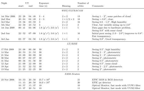
Table 1.Log of the observations.

Night UT Exposure Number of

start end time (s) Binning orbits Comments

WHT/ULTRACAM

1st Mar 2006 22 : 28 04 : 48 3 – 4 2×2 13 Seeing 1 – 2”, some patches of cloud 2nd Mar 20 : 04 04 : 49 2 – 3 1×1/2×2 18 Seeing∼0.8”, clear.

3rd Mar 19 : 56 03 : 59 3 2×2 16 Seeing 0.8 – 1.2”. High humidity 5th Mar 22 : 50 23 : 52 3 2×2 2 Clear, but variable seeing up to 2.0” 1st Jan 2009 00 : 41 03 : 06 1.8 (g′_,r′_{); 3.6 (u}′_{) 1×1 5 Data gaps due to hardware problem.}

Seeing 0.8” with some cloud

2nd Jan 22 : 52 07 : 09 1.8 (g′_,r′_{); 3.6 (u}′_{) 1×1 16 Initial poor seeing (1.0 – 2.0”) improves to 0.8”.}

Fair transparency.

3rd Jan 02 : 57 04 : 50 1.8 (g′_,r′_{); 3.6 (u}′_{) 1×1 3 Seeing 0.8”, Good transparency.} LT/RISE

17 Feb 2009 23 : 08 00 : 08 30 2×2 2 Seeing 0.5”, high humidity

14 Mar 20 : 53 21 : 53 30 2×2 2 Seeing 2 – 3”, photometric

21 Mar 23 : 09 00 : 09 30 2×2 2 Seeing 2 – 3”, photometric

30 Mar 00 : 07 02 : 07 30 2×2 4 Seeing 2”, photometric

31 Mar 00 : 56 01 : 56 30 2×2 2 Seeing 0.5”, photometric 12 Apr 21 : 09 22 : 09 30 2×2 2 Seeing 0.5”, some cloud 19 Apr 21 : 52 22 : 52 30 2×2 2 Seeing 2 – 2.5”, photometric

13 May 21 : 25 22 : 25 30 2×2 2 Seeing 2”, photometric

XMM-Newton

23 Nov 2006 10 : 53 20 : 50 35.7×103 _{21 EPIC MOS & RGS detectors}

11 : 15 20 : 50 34.0×103 _{20 EPIC pn detector}

10 : 57 15 : 37 10 10 Optical Monitor, fast mode with UVW1 filter 15 : 37 20 : 51 10 11 Optical Monitor, fast mode with UVM2 filter

with a 2×_{2 binning and the RISE V +R filter. Each}

ob-servation was 1h in length (except the obob-servation on 30 March, which was twice as long) with exposure times of 30s. The purpose of these observations was to characterise the superhump, since this exposure time is too long to ad-equately sample the eclipse. We reduced these data using aperture photometry as with the WHT/ULTRACAM data, using the ULTRACAM pipeline software.

2.3 XMM-NEWTON

SDSS 0926 was observed withXMM-Newtonon 23 Novem-ber 2006. It was observed for 34.0 ksec in the EPIC pn de-tector and 35.7 ksec in the EPIC MOS dede-tectors. It was detected with a mean count rate of 0.033±_{0.001 ct/s in the}

EPIC pn and 0.021±_{0.008 ct/s in the EPIC MOS (1+2), but}

was too faint in X-rays to be detected in the RGS detectors. The particle/X-ray background was low during the course of the observation. The Optical Monitor (OM) was configured in fast-mode and the observation time was split between the UVW1 (2450–3200˚A) and UVM2 (2050–2450˚A) filters. The source was detected with a mean count rate of 0.68 ct/s in UVW1 and 0.24 ct/s in UVM2.

The X-ray data were processed using theXMM-Newton Science Analysis Software(SAS) v9.0. For the EPIC detec-tors, data were extracted using an aperture of 30′′ centered on the source position. Background data were extracted from a source free region. The background data were scaled and subtracted from the source data. The OM data were reduced usingomfchain_.

2.4 The Catalina Real-Time Transient Survey

The Catalina Sky Survey (Larson et al. 1998) is a search for near-Earth objects using the 0.7m f /1.9 Catalina Schmidt Telescope north of Tucson, Arizona. This survey uses a sin-gle unfiltered 4k × _{4k CCD with 2.5” pixels, giving an 8}

deg2 _{field of view. The Catalina Real-Time Transient}

Sur-vey (CRTS; Drake et al. 2009) began analysing these data in real-time in November 2007 for optical transients.

The CRTS dataset contains 202 separate observations of SDSS 0926 between 10 November 2004 and 11 June 2010. Each observation is 30s in length, and they are divided up into groups of (typically) 4 observations taken over a ∼₃₀

min period. These data were reduced following Drake et al. (2009).

3 RESULTS

3.1 WHT/ULTRACAM light curves

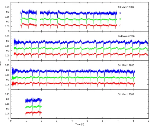
The March 2006 data are plotted in Figure 1 and the Jan-uary 2009 data are plotted in Figure 2. Additionally, we phase-folded the data on a night-by-night basis using the ephemeris given in Section 4.1, and plot the results in Figure 3. We omit from this plot the short section of data collected on 5th March 2006.

C.M. Copperwheat et al.

0 0.05 0.1 0.15 0.2

0.25 1st March 2006

u’

g’

r’

0 0.05 0.1 0.15 0.2

0.25 2nd March 2006

0 0.05 0.1 0.15 0.2 0.25

mJy _{3rd March 2006}

0 0.05 0.1 0.15 0.2 0.25

0 1 2 3 4 5 6 7 8 9

Time (h)

5th March 2006

Figure 1.Light curves of SDSS0926, observed in March 2006 with WHT/ULTRACAM. All data were collected simultaneously in the

u′_{- (top, blue),g}′_{- (middle, green) andr}′_{-bands (bottom, red). For clarity we apply offsets of 0.05mJy to theg}′_{-band data and 0.1mJy}

to theu′_{-band data. The gaps in the first night of data are due to poor weather conditions.}

so we see the peak of the superhump emission at different phases on different nights. On 1 March the peak of the su-perhump is soon after the eclipse. On 2 March it is shortly before the eclipse, and on 3 March it is not immediately apparent, but the shape of the light curve before and af-ter the eclipse suggests that the superhump and the eclipse are approximately superimposed. If we examine the eclipse feature itself, we see that the primary eclipse is immedi-ately followed by a distinct second, smaller eclipse (this is most apparent in the 3 March data). We will show in Sec-tion 4.2 that these two eclipses are of the white dwarf and the bright spot, respectively. The eclipses are preceded by a small orbital ‘hump’ caused by the bright spot moving into the field of view. This is not immediately apparent since the bright spot is relatively weak in these data, so the out-of-eclipse variation is dominated by the superhump. As well as the superhump and eclipse features we see the stochas-tic ‘flickering’ variation that is characterisstochas-tic of accreting

sources. This variation is mitigated to some degree in the phase-folded lightcurves (Figure 3). Following Smith et al. (2002) we find the mean magnitudes outside of eclipse to be 19.05±_{0.10, 19.24}±_{0.07 and 19.39}±_{0.08 inu}′_,g′ _{and r}′

respectively.

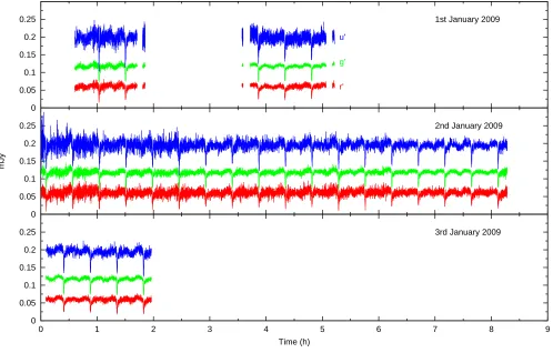
In contrast to 2006, in the 2009 data the shape of the out-of-eclipse light curve is roughly constant from night to night: we do not see the large variations caused by a super-hump component precessing through the light curve. The shape of the light curve on all three nights is most similar to the 2 March 2006 data, with the peak of the emission shortly before the eclipse. Since the position of this peak does not vary from night-to-night it is most likely due to the bright spot, and thus there seems to be no significant superhump contribution in these data. The mean magnitudes outside of eclipse are 18.94±_{0.13, 19.31}±_{0.07 and 19.43}±_{0.11 inu}′_,

g′_andr′ _{respectively, consistent with the 2006 values. Note}

0 0.05 0.1 0.15 0.2

0.25 1st January 2009

u’

g’

r’

0 0.05 0.1 0.15 0.2 0.25

mJy

2nd January 2009

0 0.05 0.1 0.15 0.2 0.25

0 1 2 3 4 5 6 7 8 9

Time (h)

3rd January 2009

Figure 2.Light curves of SDSS0926, observed in January 2009 with WHT/ULTRACAM. All data were collected simultaneously in the

u′_{- (top, blue),g}′_{- (middle, green) andr}′_{-bands (bottom, red). For clarity we apply offsets of 0.05mJy to theg}′_{-band data and 0.1mJy}

to theu′_{-band data. The gaps in the first night of data are due to poor weather conditions and a hardware fault.}

a peak at a phase of∼_{0.3 as well as the main peak at}∼_0.8.

The most likely explanation for this is that bright spot is ver-tically extended, or disc is opver-tically thin, so we are seeing emission from the bright spot all the way round the orbit.

3.2 Non-orbital variability in the ULTRACAM data

In Section 4 we use the high time resolution ULTRACAM data to make precise parameter determinations. However, first it is necessary to examine the non-orbital variabil-ity in this system. We begin by examining quasi-periodic variability in the ULTRACAM data. Secondly, it is impor-tant to characterise the superhumps present in the 2006 observations, so these features can be subtracted from the lightcurves.

3.2.1 Quasi-coherent variability

In Figure 4 we plot Lomb-Scargle periodograms (Press 2002) for the complete 2006 and 2009 g′_{-band datasets obtained}

with WHT/ULTRACAM. In the 2006 data we detect a sig-nal at a frequency of∼_{1700cycles/day (P}∼_{50s), although it}

is incoherent and spread over a wide frequency range. We estimate the quality factor (the peak centroid frequency di-vided by its full width at half maximum) of this signal to be Q∼_{4 in theg}′_{-band data. We computed the periodograms}

for each of the first three 2006 nights separately and we detected this signal every night. The signal is high in theg′

-band, and is barely detected in theu′_{band. There is possibly}

a signal at the lower frequency of∼_{1400 cycles/day in the}

2009 data, but it is much weaker than the 2006 signal. We did not find any signals in the periodograms at higher fre-quencies beyond the 5000 cycles/day range plotted in Figure 4.

Similar quasi-coherent variability was first observed in CVs some decades ago (Warner & Robinson 1972; Patterson et al. 1977), and has since been observed in many CVs and X-ray binaries (see Warner & Woudt 2008 for a recent review). The peak period of the signal we detect in the 2006 data is low for a QPO, but this may be due to the fact that the accretion disc in an ultracompact binary such as SDSS 0926 is much smaller and less massive than the disc in conventional CV systems.

3.2.2 Superhumps

Figure 5 shows g′_{-band Lomb-Scargle periodgrams in the}

C.M. Copperwheat et al.

0.00 0.02 0.04 0.06 0.08 0.10 0.12

-0.25 0.00 0.25 0.50 0.75 1.00 1.25

mJy

1st Jan 2009

-0.25 0.00 0.25 0.50 0.75 1.00 1.25 Phase

2nd Jan 2009

-0.25 0.00 0.25 0.50 0.75 1.00 1.25 3rd Jan 2009 0.00

0.02 0.04 0.06 0.08 0.10 0.12

mJy

1st Mar 2006 2nd Mar 2006 3rd Mar 2006

Figure 3.Phase folded and binned light curves, showing the superhump variation from night-to-night. In the top row we plot the first three nights of data collected in 2006. In the bottom row we plot the three nights of data taken in 2009. We plot separately the data in theu′_{- (top, blue),g}′_{- (middle, green) andr}′_{-bands (bottom, red).}

-0.5 0 0.5 1 1.5 2 2.5

2 2.5 3 3.5 4

Log(Frequency) (cycles/day)

g’-band, 2009 -0.5

0 0.5 1 1.5 2 2.5

Log(Power)

g’-band, 2006

Figure 4.Lomb-Scargle periodgrams for theg′_{-band 2006 (top)}

and 2009 (bottom) WHT/ULTRACAM datasets. We convert both the y- and x-axes to a logarithm scale, and then uniformly bin the data along the x-axis (frequency). In the 2006 dataset we see a quasi-periodic oscillation (QPO) at a frequency of∼1700 cycles/day (P=∼50s).

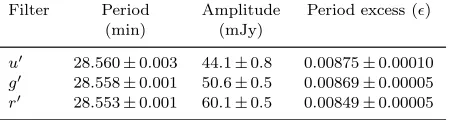
Table 2. Superhump parameters. We list the period and am-plitude of the primary sine function fitted to the complete 2006 dataset, for each of the three bands. We list also the period excess

ǫ= (PSH−POrb)/POrb, wherePSHandPOrbare the superhump

and orbital periods, respectively.

Filter Period Amplitude Period excess (ǫ)

(min) (mJy)

u′ _{28.560±0.003 44.1±0.8 0.00875±0.00010}

g′ _{28.558±0.001 50.6±0.5 0.00869±0.00005}

r′ _{28.553±0.001 60.1±0.5 0.00849±0.00005}

the eclipses of both the white dwarf and bright spot and the peak of the bright spot emission. The third panel shows the same dataset with the eclipse features unmasked but with the superhump subtracted (see below). The bottom panel shows the combined 2009 dataset, with no modification. In all four panels, vertical lines mark the positions of the su-perhump and orbital frequencies.

If the top panel of Figure 5 is examined, it can be seen that the power due to superhumps is clearly apparent, stronger than the orbital signal and peaking at a slightly lower frequency. The two signals are confused in this first panel, but the superhump is seen as being clearly distinct in the second panel, in which the majority of the orbital modulation is masked.

0.0 0.2 0.4 0.6 0.8 1.0

46 48 50 52 54

Power

Cycles/day 2009, unmodified

0.0 0.2 0.4 0.6 0.8 1.0

2006, with superhump subtracted

0.0 0.2 0.4 0.6 0.8 1.0

2006, with eclipse masked

0.0 0.2 0.4 0.6 0.8 1.0

2006, unmodified

Figure 5.Lomb-Scargle periodograms for theg′_{band data. We}

plot the power around the orbital frequency, with the peak of each distribution normalised. The vertical lines mark the frequency of the superhump (blue, dotted) and the orbital (red, solid) mod-ulations. The four periodograms are (from top to bottom): (i) The 2006 data, showing both the superhump and orbital modu-lations. (ii) The 2006 data with the eclipse and bright spot fea-tures masked. (iii) The 2009 data with the superhump subtracted, using the method described in Section 3.2.2. (iv) The 2009 data.

to fit any residual signal left after the masking of the eclipse features. In the third panel of Figure 5 the periodogram for the unmasked dataset with the superhump components sub-tracted is plotted. We see that our model fits do a good job of cleaning the superhump signal from the data.

Our findings for the superhump period are listed in Table 2. The uncertainties on these periods were deter-mined from fits to a series of sample datasets derived from the originals using the bootstrap method (Efron 1979; Efron & Tibshirani 1993). The amplitudes of the superhump harmonics are< 10% of the amplitude values for the pri-mary frequency. We find the period of the variation to be consistent at the 1σlevel for theu′_{- andg}′_{-bands, but the}

r′

-band period is lower. This inconsistency is probably due to some extra intrinsic variability, such as accretion-driven flickering. The amplitude of the modulation increases at longer wavelengths. We list also in this table the period excesses ǫ in each band, using the orbital period given in Section 4.1.

Finally, the fourth panel of Figure 5 shows the 2009 data. This plot shows a clean signal at the orbital frequency, confirming that there is no superhump modulation in these data. Following these observations, we obtained a series of 1h light curves using LT/RISE over the first half of 2009. The purpose of these observations was to examine the long term behaviour of the superhump, although with hindsight they were perhaps too short. Two of these light curves were in the immediate aftermath of an outburst in this system, and we will discuss these separately in Section 3.3.1. Of the remaining light curves, few show clear evidence for the su-perhump. On 17 February and 21 March there is a ‘hump’ just before the eclipse, but this could be due to the bright spot. Most of the remaining quiescent light curves show lit-tle out-of-eclipse variation. One exception is the light curve obtained on 19 April, which shows a clear brightening imme-diately following the eclipse, which can only be explained by the superhump. This light curve was obtained 21 days after the detection of the outburst in this system. There was no clear evidence for the superhump obtained seven days prior to this one, on 12 April.

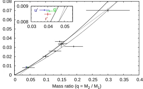
Patterson et al. (2005) suggestedǫ= 0.18q+ 0.29q2 _as

an empirical relationship between the superhump period ex-cess ǫ = (PSH −POrb)/POrb, and the mass ratio q. This

relationship was calibrated using measurements of a series of eclipsing systems, listed in Table 7 of Patterson et al. (2005). The relation is pinned by settingǫ= 0 whenq= 0, but this is an assumption and not empirically determined: of the calibration systems only KV UMa has a mass ra-tio < 0.05 and this determination is very uncertain, and so the calibration is potentially poor at low mass ratios. SDSS 0926 is therefore potentially a strong test of this re-lationship, although it has been argued that it would not apply to AM CVn systems (Pearson 2007). In Figure 6 we reproduce Figure 1 from Patterson et al. (2005), adding our measurements from the 2006 data in u′

, g′

and r′

, using the values given in Tables 2 and 6. As well as the Pat-terson relation, we also plot the slightly modified relation proposed by Kato et al. (2009) (ǫ= 0.16(2)q+ 0.25(7)q2₎

and the linear relation proposed by Knigge (2006) (q(ǫ) = (0.114±_0.005)+(3.97±_0.41)×_(ǫ−_{0.025)). The Knigge}

C.M. Copperwheat et al.

0 0.01 0.02 0.03 0.04 0.05 0.06 0.07 0.08

0 0.05 0.1 0.15 0.2 0.25 0.3 0.35 0.4

Period excess (

ε

= [P

SH

- P

orb

] / P

orb

)

Mass ratio (q = M₂ / M₁)

0.008 0.009

0.03 0.04 0.05

r’ g’

u’

Figure 6. Mass ratioqversus the superhump period excess ǫ. The blue, green and red points show our u′_{-, g}′_{- and r}′_-band

determinations, respectively. The region around these points is magnified in the inset. The solid line is the ǫ= 0.18q+ 0.29q2

relationship proposed by Patterson et al. (2005). The dashed line is theǫ= 0.16q+ 0.25q2_{relation proposed by Kato et al. (2009).}

The dotted line is the linearq(ǫ) = (0.114±0.005)+(3.97±0.41)×

(ǫ−0.025) relation proposed by Knigge (2006). The black points are the eclipsing CVs listed as calibration sources in Table 7 of Patterson et al. (2005).

these relations to within their uncertainties, and are closest to the Patterson et al. (2005) relation, which suggests the assumption ofǫ= 0 whenq= 0 is reasonable.

3.3 Outbursting behaviour

The superhumps are a transient phenomenon that is driven by outbursts, so here we examine the outbursting history of this system, presenting the first observations of SDSS 0926 in outburst. We begin by discussing observations taken with the LT in the immediate aftermath of an outburst in March 2009. We go on to examine the long-term outbursting be-haviour using five years of CRTS observations.

3.3.1 The March 2009 outburst

On 29 March 2009 it was discovered that SDSS 0926 was in outburst. We obtained 2h of data with LT/RISE on the subsequent night, and a further 1h on the night after that. We plot these data in Figure 7. The flux scale for these data is such that the mean, quiescent out-of eclipse flux is equal to 1. We also plot the model fit (described in Section 4.2, below) to our quiescent superhump subtracted LT/RISE ob-servations for comparison. We apply an arbitrary flux offset to this model light curve so as to overlay it on the outburst data. We see that at the beginning of our 30 March obser-vation the system was a factor of∼_{3.5 brighter than during}

quiescence and declining quickly: this has dropped to a fac-tor of 3 by the end of the 2h observation. The following night this has dropped to a factor of 2. There is still some evidence of the outburst in our next observation on 12 April: the out-of-eclipse flux in this light curve is ∼_{10% greater than the}

mean level.

We phase-folded the 30 March data using the ephemeris given in Section 4.1, and plot the results in Figure 8. Again,

we plot a quiescent model light curve for comparison. In this plot the structure in the light curve after the outburst is more evident. There are two main features: the primary eclipse centred on a phase of 0, and a separate, smaller dim-ming in the light curve centred on a phase of∼−_{0.25. If we}

examine the primary eclipse first we see it is much deeper and wider than the quiescent white dwarf eclipse. The eclipse width is consistent with this being an eclipse of the accre-tion disc. The eclipse is asymmetric however, and there is a clear ‘step’ in the egress. This suggests an uneven distribu-tion of flux over the surface of the accredistribu-tion disc itself, or (perhaps more likely) this step could be due to the bright spot. The step height of this egress is much larger than the bright spot egress during quiescence however, and so if this feature is attributed to the spot it would imply an enhanced mass transfer during the outbursting state, or an increased viscous heating at the bright spot position.

The second unusual feature in the phase-folded light curve is the dimming centred on a phase of ∼−_{0.25. This}

dimming begins at approximately the same time that the bright spot begins to come into view in the quiescent light curve. The phase of this feature is such that the eclipsing component cannot be either the white dwarf, the donor or the bright spot. We suggest this feature may be due to a warped accretion disc (Pringle 1996), the distortion being induced by the outburst. The dimming we see can therefore be explained by obscuration of the white dwarf or inner disc by the accretion disc itself. This is a very short lived fea-ture: we see no evidence for it in the data collected on the subsequent night.

Finally, as we discussed in Section 3.2.2 we detect su-perhumps in this system in data obtained 21 days after the outburst. This is consistent with the expectation that, since the superhumps in this system are not permanently present, they are induced by the perturbation of the disc by the out-burst.

3.3.2 Long-term variations

We plot in Figure 9 the unfiltered data collected by the Catalina Real-Time Transient Survey (CRTS). These data were collected between 10 November 2004 and 11 June 2010. We observe a total of either six or seven outbursts in these data, but the time sampling is such that they do not give an exhaustive picture of the outbursting behaviour of the source over this time period: there are no observations around the time of the March 2009 outburst, for example, and so this outburst is missed. Note that we do detect an outburst∼₂₅

days before the 2006 ULTRACAM observations. It is likely that this outburst induced the superhumps we see in these data by perturbing the disc.

The CRTS data is split up into blocks of four 30s ob-servations taken over a ∼_{30 min period. There is typically}

1.8 2 2.2 2.4 2.6 2.8 3 3.2 3.4 3.6

0.01 0.02 0.03 0.04 0.05 0.06 0.07 0.08 0.09

Flux

MJD - 54921 (days) 0.8

1 1.2 1.4 1.6 1.8 2 2.2 2.4 2.6

1.05 1.06 1.07 1.08

Figure 7.LT/RISE light curves obtained on 30 and 31 March 2009: one day and two days after an outburst in this source was first detected, respectively. We plot these data in flux units, with the mean quiescent out-of-eclipse flux set to unity. The solid red line is a model fit to our quiescent, superhump-subtracted LT/RISE observations with an arbitrary flux offset, which we plot for comparative purposes.

1.8 2 2.2 2.4 2.6 2.8 3 3.2 3.4 3.6

-0.5 -0.4 -0.3 -0.2 -0.1 0 0.1 0.2 0.3 0.4 0.5

Flux

Phase

Figure 8.The LT/RISE data collected one day after the March 2009 outburst, phase-folded using the ephemeris given in Section 4.1. We plot these data in flux units, with the mean quiescent out-of-eclipse flux set to unity. The solid red line is the quiescent, superhump-subtracted model light curve with an arbitrary flux offset, which we plot for comparative purposes.

ever, outbursts of∼_{12 days have been observed in KL Dra,}

aP= 25 min AM CVn system (Ramsay et al. 2010). The mean magnitude of the quiescent, out-of-eclipse points is 19.33±_{0.31. The outbursts range in magnitude}

from 17.11±_{0.08 to 16.81}±_{0.12. Note that for all six}

out-bursts it is unclear how much time has elapsed between the initial rise and the observation, and so these measurements set a lower limit on the peak brightness. Our LT/RISE ob-servations of the March 2009 outburst showed a factor ∼₃

enhancement in flux a day after the initial detection, and a factor ∼_{2 enhancement a day after that. This is relatively}

modest compared to the outbursts observed in the CRTS data. We conclude that the March 2009 outburst was a rel-atively minor one for this source. An outburst of this size would only be detectable in the CRTS data within 1 – 2 days of the initial rise. The average outburst recurrence time is therefore difficult to determine. If we exclude the two out-bursts which occur within 8 days of each other the time be-tween observed outbursts ranges from 104 to 449 days, but since we may have missed a number of outbursts the actual

16

17

18

19

20

21

22

0 500 1000 1500 2000 2500

Magnitude (unfiltered)

MJD - 53200 (Days) 2006 obs. 2009 obs.

Figure 9.Observations made by the Catalina Real-Time Tran-sient Survey (CRTS). These data were collected between 10 November 2004 and 11 June 2010, and six outbursts were ob-served over that period. The solid lines at the top of the plot indicate the times of the 2006 and 2009 observations with the WHT and LT.

recurrence time may be shorter. For comparison, an outburst cycle of∼_{60 days was observed in KL Dra (Ramsay et al.}

2010).

3.4 XMM-Newton observations

C.M. Copperwheat et al.

NH 1.3±0.3×1021cm−2

α 1.8+∞

−0.5

kTmax 30 keV (fix)

Observed flux 0.1-10keV 1.2+2−0..83×10−13erg s−1 cm−2

Unabsorbed

bolometric flux 2.7+5−0..88×10

−13_{erg s}−1 _cm−2

Unabsorbed

bolometric luminosity 3.2+6.8

−0.9×1029erg s−1d2100

χ2

ν=1.03 (103 dof)

Table 3. The X-ray spectral fit parameters derived using a si-multaneous fit to the EPIC pn and MOS spectra.

3.4.1 X-ray data

We extracted light curves from the EPIC pn and both EPIC MOS cameras and combined them into one light curve, which was folded using the ephemeris given in Section 4.1. We found no evidence for an eclipse in the X-ray light curve. To investigate this further we searched for periods using a Discrete Fourier Transform and phase dispersion methods and found no clear signal of an eclipse.

Using the original X-ray light curve as a benchmark, we added an eclipse of given depth to the light curve. We gen-erated 100 light curves for a given eclipse depth. We found that for a partial eclipse with a depth of<90%, we would likely not detect the eclipse. Even for a total eclipse we would have only a 70% probability of detecting the eclipse.

We extracted integrated X-ray spectra from the EPIC pn and MOS detectors (with corresponding background spectra) and fitted them simultaneously using an absorbed thermal plasma model. Unlike other AM CVn systems (Ramsay et al. 2005, 2006), we found that varying the metal abundance did not significantly improve the goodness of fit (probably since the signal-to-noise ratio of the spectra was relatively low). We obtained a good fit to the data, and the derived spectral parameters are listed in Table 3.

The best-fit value for the absorption is high (1.3±_0.3×

1021_cm−2_{) for an object at a high galactic latitude (+46}◦_).

In contrast, the absorption to the edge of the Galaxy is

∼ _1.4× ₁₀20 _cm−2_{(Dickey & Lockman 1990). If we fix}

the column density parameter in the spectral fits to the Dickey & Lockman (1990) value the resulting fit (χ2

ν=1.96,

104 dof) was poorer at a confidence level of > 99.99%. If this ‘extra’ absorption originates in SDSS 0926 itself it may be due to viewing the boundary layer through the disc, since the binary inclination is high. Finally, we calculate the unab-sorbed bolometric X-ray luminosity using the distance given in Section 5.2, and find it to beLx= 6.9×1030erg s−1.

3.4.2 Ultraviolet data

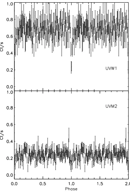
We binned the OM light curves into 5s bins and folded them on the ephemeris given in Section 4.1. The resulting light curve is plotted in Figure 10. The eclipse is clearly seen in the UVW1 filter, where the count rate is consistent with zero atφ=0.0 in a single bin. In the shorter wavelength fil-ter, UVM2, the signal-to-noise ratio is lower, but there is some evidence for a dip at φ=0.0, although it is not to-tal. We searched for other periods using a Discrete Fourier

Figure 10.Phase folded UV lightcurves obtained using

XMM-Newton_{OM. The top and bottom plots are through the UVW1}

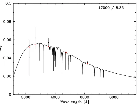
Figure 11.We determine the white dwarf temperature by fit-ting our measurements of the white dwarf flux in the optical and UV to a library of synthetic spectra (G¨ansicke et al. 1995). The spectrum we plot here is for a 17,000K white dwarf, and is the best fit to our flux determinations. The numbers in the top right corner are the temperature and loggfor the model fit.

Transform (Deeming 1975) and phase dispersion methods (Stellingwerf 1978) and found no other significant periods in the light curves.

We derived UV fluxes by converting the count rate in the two UV filters to a flux by assuming a conversion fac-tor which was derived using observations of white dwarfs usingXMM-NewtonOM. A mean count rate of 0.71±_0.02

ct/s in the UVW1 filter corresponds to a flux of 3.2×₁₀−16

erg s−1 _cm−2_{/˚A, while 0.27±0.01 ct/s in the UVM2 filter}

corresponds to a flux of 5.3×₁₀−16_{erg s}−1_cm−2_{/˚A. We}

cal-culate the ultraviolet luminosity following the approach of Ramsay et al. (2005, 2006), by assuming a blackbody flux distribution and fixing the normalisation to give the inferred de-reddened ultraviolet flux in the two filters. This gives an ultraviolet luminosity of Luv = 1 – 3×1032erg s−1. Both

this luminosity and the X-ray luminosity Lx, given in the

previous section, are consistent with the findings for other AM CVn systems of similar period (Ramsay et al. 2006).

We used the UV and optical fluxes to determine the effective temperature of the white dwarf, by estimating the contribution of the white dwarf in each band. In the three ULTRACAM bands this parameter is determined through our model fits, as discussed in Section 4. In the UV data we estimated the white dwarf contribution from the eclipse depth. We made a correction to compensate for the fact that the eclipse is only partial, by determining the frac-tion of the white dwarf’s surface area that is obscured dur-ing the eclipse in our optical fits. This correction is small though, as evidenced by the fact that the UVW1 flux reaches zero during the eclipse, within the errors. We calculated the white dwarf contributions to be UVM2∼_0.04±_{0.02, UVW1} ∼_0.062±_{0.012, u}′ _{= 0.057±0.005, g}′ _{= 0.046±0.002}

and r′ _{= 0.035±0.002 mJy. We then fitted these fluxes}

with the white dwarf model atmospheres introduced in G¨ansicke et al. (1995). We find a white dwarf temperature of 17,000K to be consistent with our measurements (Fig-ure 11). Note that in making this estimate we have not ap-plied an extinction correction to these fluxes. As we noted

in Section 3.4.1, the galactic E(B −_{V) is negligible, but}

we measure some extra absorption in the X-ray data. This is probably related to the high inclination of this system and due to our looking through a significant amount of gas above the accretion disc. Similar effects are seen in a number of CVs, such as V893 Sco (Mukai et al. 2009). This mate-rial will not be in the form of dust and so will not cause ‘extinction’ in the classical sense, but it is possible that it may cause an ‘accretion curtain’ in this system, such as in OY Car (Horne et al. 1994). If this was the case then our temperature determination was a lower limit. However, it is impossible to detect such an effect without UV spectroscopic data. Our temperature determination for the white dwarf is consistent (within the uncertainties) with the theoretical models of Bildsten et al. (2006), which predict a tempera-ture of 18,000K for this system.

4 LIGHT CURVE ANALYSIS

In this section we describe the model we fitted to the phase-folded and binned WHT/ULTRACAM 2006 and 2009 data in order to make parameter determinations for this system. For the 2006 data it was first necessary to subtract the night-to-night variations caused by the superhump; this is detailed in Section 3.2.2. Secondly, we fitted the data on an eclipse-by-eclipse basis in order to refine the ephemeris, which we discuss in Section 4.1. We then phase-folded the data using this ephemeris and fitted it with a Markov Chain Monte Carlo (MCMC) light-curve model in order to obtain final parameter determinations. We fit the three bands separately. This fitting process is described in Section 4.2.

4.1 Determination of the ephemeris

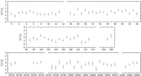
We divided each light curve into separate orbital cycles, and then fit the model determined in Section 4.2 to each cycle using the Levendburg-Marquardt method (Press 2002) in order to generate a series of eclipse timings. These timings are on the barycentric dynamical timescale, corrected for light travel to the solar system barycentre. A least-squares fit to all of these data yields the ephemeris

M JD(T DB) = 53795.9455191(5) + 0.01966127289(2)E

for the mid-point of the white dwarf eclipse. We plot the residuals of the linear ephemeris in Figure 12. There is some systematic variation, perhaps due to the residuals of the su-perhump or flickering. With only two epochs of observation any long-term departure from a linear ephemeris cannot be determined: a third epoch of high-speed observation will be necessary to identify any period changes in this system.

4.2 Fitting the phase-folded light curves

C.M. Copperwheat et al.

-3 -2 -1 0 1 2 3

52744 52746 52748 52750 52752

O-C (s)

52794 52796 52798 52800 52802 52804 52806 52808 52810 52812 Cycle

52854 52856 52858 -3

-2 -1 0 1 2 3

96 98 100 102 104 106 108 110 112 114

O-C (s)

204 206 -3

-2 -1 0 1 2 3

0 2 4 6 8 10 12 14

O-C (s)

46 48 50 52 54 56 58 60 62 64

Figure 12. (O− C) values plotted against cycle number, using the eclipse timings determined from the model fits to our WHT/ULTRACAM data and the linear ephemeris given in Section 4.1. Cycle 0 corresponds to the first eclipse in the 1 March 2006 dataset. Note the break in the x-axis of this plot between the various nights of data.

this second epoch of data. Once the superhump was sub-tracted it became clear that other binary parameters var-ied over the course of our observations, in particular the disc radius which changes significantly from night to night. These variations prevented us from combining our entire WHT/ULTRACAM dataset. We therefore chose to create separate phase-folded light curves for each individual night of observation. Even this could potentially introduce some systematic effect on our results due to the change in disc radius between the beginning and end of each night’s obser-vation. We examine this in detail in Section 5.4 and find that such effects are small, so we do not believe this influences our results to a significant degree. Since we cannot com-bine nights, we chose to omit the nights of 5 March 2006, 1 January 2009 and 3 January 2009, in which we only have a few cycles of data. We therefore fitted a total of twelve light curves: theu′

-,g′

- and r′

-band phase-folded data for the nights of 1, 2 and 3 of March 2006; and 2 January 2009.

We modelled the light curve with LCURVE, a code

de-veloped to fit light-curves characteristic of eclipsing dwarf novae and detached white dwarf / M dwarf binary stars. A complete description of this code is given in the appendix of Copperwheat et al. (2010). We implemented this code in this work with two modifications, both to the bright spot component. In Copperwheat et al. (2010) the bright spot is modelled as a line of elements which lie upon a straight line in the orbital plane. The surface brightness of the elements is parameterised with two power-law exponents. Since the bright spot in SDSS 0926 is a relatively weak component

of the emission we do not require this degree of complexity. We therefore use a simpler bright spot model, setting the exponentγto 1 (our bright spot model is therefore identical to the earlier prescription of Horne et al. 1994). Secondly, in Copperwheat et al. (2010) the angleφwas defined as the angle the line of elements of the bright spot makes with the line of centres between the two stars. We have changed the definition of this angle in our code:φis now the angle the line of elements of the bright spot makes with the tangent to the outer edge of the accretion disc. This modification makes this angle easier to interpret in a physical context, sinceφ= 0 implies a bright spot which runs along the outer edge of the disc, and so we would expectφ to be close to this. We noted in Copperwheat et al. (2010) that the two anglesφ andψ (the angle away from the perpendicular at which the light from the bright spot is beamed) are highly correlated and tend to be poorly constrained, and so here we fixφ= 0.

In theLCURVEcode the binary is defined by four

Table 4.Limb darkening coefficients for the primary white dwarf, using the four-coefficient law of Claret (2000).

Coefficient u′ _g′ _r′

1 1.35 1.18 1.37 2 −1.30 −1.13 −2.07 3 0.90 0.75 1.96 4 −0.28 −0.23 −0.72

toRspot: the distance between the bright spot and the

pri-mary white dwarf. We therefore assume that the ‘head’ of the bright spot is on the outer rim of the disc. Rdisc is

rather poorly constrained by our data, and as we showed in Copperwheat et al. (2010)Rspotis highly correlated with

Rdisc, so this is a reasonable approximation. One additional

parameter which our results are potentially sensitive to is the limb darkening of the primary white dwarf. We made an initial fit to the data in order to estimate the effective temperature and surface gravity (we discuss these quanti-ties in Section 5.2), and then used a model atmosphere code (described in Koester 2010) to calculate the specific inten-sity at different points across the stellar disc. We then fitted these values to determine the limb darkening coefficients. We tried various limb darkening laws, and found the best fit was for the four-parameter law of Claret (2000), although the choice between this and a fourth order polynomial is unlikely to influence our results. We list our determinations of the coefficients in Table 4. These values were used in all our MCMC fits.

The parameter determinations from these fits are listed in Table 5. Note that the uncertainties on these MCMC re-sults are non-Gaussian, and so the values we quote in this table only provide an approximate description of the un-certainties. We plot the distribution of the mass ratio and inclination values from our fits in Figure 14. Additionally, in Figure 13 the phase-folded light curves for the four nights are plotted, along with the best model fits. If we examine Figure 13 first, we see we obtain a good fit to the data in all three bands for each of the four nights. The dominant component in the light curve is the primary white dwarf, and the main eclipse in the light curve is the eclipse of this feature. Note that the eclipse is round-bottomed, meaning it is a partial eclipse of the white dwarf. The second, smaller eclipse in these light curves is of the bright spot, which is a much weaker component. The phase of this eclipse clearly varies with respect to the phase of the white dwarf eclipse: this can be understood in terms of a change in the relative position of the bright spot due to variations in the disc ra-dius. Compare for example the first night of 2006 with the second. On the first night, the two eclipses are clearly dis-tinct, with the egress of the white dwarf followed by the ingress of the bright spot. On the second night, the egress and the ingress overlap. This implies a larger apparent ac-cretion disc radius on the second night, due to the precession of the elliptical disc. The two other nights of data lie some-where between these two extremes. The fact that the two eclipses are sometimes separate implies a very low mass ra-tio for this system: in higher mass rara-tio systems we would expect to see the ingress of both the white dwarf and the bright spot before the white dwarf egress.

We now turn to the parameter determinations listed in

Table 5. The first four of these are the parameters that are important in characterising the system: these are the mass ratio q, the binary inclination i, the primary white dwarf radius scaled by the binary separation R1/a, and the

ac-cretion disc radius scaled by the binary separationRdisc/a.

The mass ratio and the inclination are highly correlated, and we discuss these parameters in Section 5.1. The white dwarf temperature is used withq,iandR1/ato derive the

remaining binary parameters in Section 5.2. We discuss the disc radius in more detail in Section 5.4. The remaining six parameters in Table 5 pertain to the accretion disc and the bright spot. We find these parameters to be rather poorly constrained in general, due to the fact that the disc and the bright spot make a relatively weak contribution to the flux in this system. However, we find no correlation between these parameters and the ‘important’ parameters listed above, and so the uncertainty in these values does not imply any further systematic uncertainty in the determinations of Sections 5.1 and 5.4.

5 DISCUSSION

5.1 Mass ratio and inclination

If we assume a Roche-lobe filling donor star, the phase width of the white dwarf eclipse is then an observable quantity that is intrinsically linked to two physical properties: the mass ratio and the binary inclination. For a higher binary inclination the duration of the eclipse will be greater, thus to maintain the same phase width, as the inclination is in-creased, the size of the donor, and hence the mass ratio, must be decreased. There is therefore a unique relationship between these two properties (Bailey 1979). This degener-acy can be broken since we have an additional geometric constraint due to the ingress and egress of the bright spot. The path of the accretion stream and hence the position of the bright spot is modified by the mass ratio. With this ad-ditional information we can determine both the mass ratio and inclination in this system.

Our MCMC results for the mass ratio versus inclination are plotted in Figure 14. We see that these points are dis-tributed along a curved path across this plot: this is the line of constant phase width for the white dwarf, which we mea-sure to be∼_{0.0220. The points are constrained to this line,}

with the scatter due to the uncertainty in the phase width. We calculate the weighted means of theq,iandR1/avalues

in Table 5, and present the results in Table 6. We emphasise at this point that the weighted means may underestimate the uncertainties in these parameters. The MCMC results in Table 5 show variations which are formally significant, most likely due to effects such as flickering and residuals from the superhumps. In addition, the bright spot compo-nent is weak in this system, and so the best fit model for this component can be quite different in different bands, partic-ularly inu′_{. It is important therefore to note that the results}

we discuss in this and the following sections, and in Table 6, may not fully account for these systematic effects, and the magnitude of these effects are better understood by referring to the individual night’s results in Table 5.

We find the mass ratioM2/M1to beq= 0.041±0.002 in

ourg′

C.M. Copperwheat et al.

0.01 0.03 0.05 0.07 0.09 0.11

mJy

Mar 2006, night 1 u’

g’

r’

Mar 2006, night 2

0.01 0.03 0.05 0.07 0.09 0.11

mJy

Mar 2006, night 3 Jan 2009, night 2

-0.15 -0.10 -0.05 0.00 0.05 0.10 0.15

Phase

-0.15 -0.10 -0.05 0.00 0.05 0.10 0.15

White dwarf

Bright spot Accretion disc

Figure 13.Phase-folded and binned light curves for the first, second and third nights of the 2006 observations, and the second night of the 2009 observations. For each we plot the three bands separately (top,u′_{; middle,g}′_{; bottom,r}′_{). We plot the average flux in mJy}

against the binary phase, where a phase of 0 corresponds to the mid-eclipse of the white dwarf. We plot the datapoints with uncertainties in black, and the best model fits to these data in blue, green and red (foru′_,g′ _andr′_{, respectively). For clarity we apply offsets of}

0.005mJy to theg-band data and 0.01mJy to theu-band. For each night we also show underneath the lightcurve the three components of theg′_{-band model plotted separately, showing the relative strengths of the bright spot, accretion disc and white dwarf. These three}

lines have also been offset for clarity.

deg ing′_{. The values ofq andiin the other two bands are}

consistent with these values. Our 2006 data were originally published in Marsh et al. (2007) and there we reported dif-ferent values of 0.035±_{0.002 and 83.1}±_{0.1 deg forq and}

i. This discrepancy is due to a number of factors. Primar-ily, the MCMC method we use for minimisation is supe-rior to the Levenberg-Marquardt minimisation employed in Marsh et al. (2007). We have found in situations of strong degeneracy, such as between q and ihere, the Levenberg-Marquardt and simplex methods have a tendency to stop before finding the true minimum (Copperwheat et al. 2010). Additionally, we have used more appropriate limb-darkening coefficients in this work, since we have been able to estimate the white dwarf temperature. Marsh et al. (2007) also ar-rived at their parameter determinations by combining data from different nights, which as we have discussed may

intro-duce some systematic uncertainty due to the changing disc radius.

5.2 Other binary parameters

In Table 6 we list our determination of the primary white dwarf radius, scaled by the binary separation. We used this, combined with our determination of the mass ratio and the binary inclination, to calculate the remaining binary param-eters. One additional piece of information that was needed for this is a mass/radius relation for the primary white dwarf.

Figure 14.The distribution of the mass ratioqand inclinationiresults from our MCMC runs, with the green and red regions indicating the 1σand 3σ confidence intervals. We plot (from left to right) nights 1, 2 and 3 of the 2006 observations, and night 2 of the 2009 observations. For each night we plot (top to bottom) the distribution in theu′_,g′ _andr′_bands.

relation for the white dwarf, and for this we used the Eggleton zero-temperature mass/radius relation (quoted in Verbunt & Rappaport 1988). We subsequently determined the mass and radius of the white dwarf, and from our model calculated the white dwarf contribution in each band. It is these white dwarf fluxes which we list in Section 3.4.2. We then used the white dwarf model atmospheres of G¨ansicke et al. (1995) to calculate the white dwarf temper-ature Tef f, fixing logg to the value implied by the

zero-temperature mass and radius. We then compared these val-ues of Tef f and M1 to the white dwarf cooling models of

Bergeron et al. (1995) in order to find the white dwarf ra-dius which is consistent with these values. By comparing this to the Eggleton zero-temperature radius, we determined an ‘oversize factor’ for the white dwarf, which we found to be 1.03. Finally, we determine a final white dwarf mass and radius using a new mass/radius relation, which is the zero-temperature relation scaled by this oversize factor. In theory, at this point we should then re-iterate this process and use the new mass and radius to refine the temperature determi-nation. However, since the first oversize factor is very close to 1 the effect of further iterations is negligible: the white dwarf

temperature fit is not affected by the very small change in logg which results from a 3% increase in the white dwarf radius. Note also that since the oversize factor is so close to 1, while the uncertainty in our temperature measurement may be quite large (since it is based on a small number of flux measurements) it will not affect our parameter deter-minations to a significant degree.

In the second half of Table 6, we list the binary

separa-tiona, the masses of the two components, the radial

veloc-ity semi-amplitudes of the two components and the radius of the secondary. This radius is the volume radius of the Roche lobe filling donor, which we calculate using the approxima-tion of Eggleton (1983). In ourg′_{-band fits, we find the mass}

of the primary white dwarf to be 0.85±_{0.04M⊙. The mass}

of the donor is 0.035±_{0.003M⊙ and the donor radius is}

0.047±_{0.001R⊙. In Marsh et al. (2007), we reported the}

primary mass to be 0.84±_{0.05M⊙ and the donor mass to}

be 0.029±_{0.002M⊙. These values are close to our updated}

C.M. Copperwheat et al.

Table 5.Results from our MCMC fits to the phase-folded light curves, as detailed in Section 4.2. q: the mass ratio. i: the bi-nary inclination.R1: the white dwarf radius.Rdisc: the accretion

disc radius. β: the power-law exponent for the bright spot. δ: the exponent of surface brightness over the accretion disc.l: the bright spot scale-length.fc: the fraction of the bright spot taken

to be equally visible at all phases.φ: the angle made by the line of elements of the bright spot, measured in the direction of bi-nary motion from the line tangental to the accretion disc.ψ: the angle away from the perpendicular at which the light from the bright spot is beamed, measured in the same way asφ. A com-plete description of all these parameters is given in the appendix of Copperwheat et al. 2010

u′ _g′ _r′

2006, night 1

q 0.037±0.003 0.051±0.004 0.043±0.003

i 82.94±0.29 81.89±0.25 82.53±0.23

R1/a 0.037±0.004 0.036±0.001 0.027±0.002

Rdisc/a 0.341±0.013 0.336±0.049 0.339±0.012

δ −1.86±0.55 −2.23±0.39 −1.99±0.22

l 0.040±0.006 0.026±0.002 0.018±0.004

fc 0.914±0.018 0.846±0.024 0.921±0.012

β 2.04±1.00 2.51±0.76 2.25±1.01

ψ 22.5±15.2 172.1±12.7 21.4±7.7

2006, night 2

q 0.038±0.002 0.046±0.003 0.042±0.002

i 82.58±0.22 82.13±0.28 82.52±0.19

R1/a 0.040±0.001 0.034±0.001 0.035±0.002

Rdisc/a 0.455±0.012 0.415±0.013 0.435±0.008

δ −0.71±0.32 −1.90±0.21 −0.80±0.22

l 0.002±0.003 0.011±0.003 0.004±0.002

fc 0.636±0.014 0.79±0.02 0.67±0.02

β 1.54±1.05 2.02±0.97 1.39±1.11

ψ 46.8±7.1 37.0±6.3 39.6±9.9

2006, night 3

q 0.039±0.001 0.039±0.002 0.037±0.002

i 82.77±0.16 82.80±0.21 82.89±0.18

R1/a 0.036±0.001 0.037±0.002 0.032±0.002

Rdisc/a 0.394±0.009 0.369±0.004 0.370±0.004

δ −0.68±0.19 −0.88±0.28 −1.40±0.28

l 0.069±0.001 0.026±0.004 0.024±0.002

fc 0.916±0.005 0.91±0.01 0.91±0.01

β 0.92±0.29 3.00±0.62 3.10±0.55

ψ 29.0±13.6 24.6±8.2 23.9±7.3

2009, night 2

q 0.028±0.004 0.040±0.001 0.042±0.006

i 84.04±0.45 82.71±0.08 82.80±0.45

R1/a 0.043±0.003 0.032±0.001 0.015±0.005

Rdisc/a 0.289±0.012 0.393±0.002 0.379±0.019

δ 1.10±1.27 −1.89±0.12 −1.92±0.17

l 0.174±0.006 0.029±0.002 0.055±0.015

fc 0.95±0.01 0.82±0.01 0.69±0.12

β 2.62±0.74 2.34±0.51 1.12±2.76

ψ 30.43±12.1 22.9±3.4 20.4±27.0

contribution, along with the theoretical absolute magnitudes from the Bergeron et al. (1995) and Holberg & Bergeron (2006) cooling models, we can estimate the distance mod-ulus for this system. Using the absolute magnitudes for a white dwarf temperature of 17,000K and mass of 0.8M⊙,

our flux measurements imply a distance of 460 – 470pc.

5.3 AM CVn formation scenarios

A donor mass of 0.035±_{0.003M⊙ implies the donor is}

only partially degenerate: a fully degenerate donor in a system with this period would have a mass of ∼_0.020M⊙.

Roelofs et al. (2007) measured the masses of five systems us-ing parallax measurements obtained withHST, and found four of the five to be consistent with a partially degenerate donor. The degree of degeneracy varied, but the donor was typically found to have a mass of between 2 and 4 times the mass of a fully degenerate donor. The lowest estimate was for HP Lib, which was found to have a donor mass of 1.6 – 2.9 times the fully degenerate mass. At 1.75 times the fully degenerate mass, SDSS 0926 is by comparison at the lower end of these estimates.

We now examine the finding of a donor mass of 0.035±

0.003M⊙ in the context of the evolutionary history of this

system. There are three proposed formation paths for AM CVn binaries and all three are consistent with a donor that is partially degenerate to some degree. The ‘white dwarf channel’ (Nelemans et al. 2001) suggests detached close double white dwarfs which are brought into contact as a result of angular momentum loss due to gravitational wave radiation (GWR). Nelemans et al. (2001) used a zero-temperature donor in their formulation, but Deloye et al. (2005) argued that the donors could be semi-degenerate to some degree, depending on the contact time of the bi-nary. The second formation path is the ‘helium star chan-nel’ (Iben & Tutukov 1991). In this scenario the donor is a low-mass, non-degenerate helium burning star. Follow-ing contact, material is accreted from the helium star onto the primary white dwarf until a donor mass of∼_0.2M⊙is

reached, at which point core helium burning ceases and the star becomes semi-degenerate. Further mass transfer driven by GWR sees the donor mass decrease and the orbital pe-riod increase to values consistent with the observed AM CVn population. The third scenario is the ‘evolved CV channel’ (Podsiadlowski et al. 2003) which suggests the progenitors of AM CVns are CVs with evolved secondaries. The donor in this channel is initially non-degenerate and hydrogen-rich, but becomes degenerate and helium-rich (but still with a few per cent hydrogen) during its evolution before Roche lobe overflow.

Nelemans et al. (2001) approximated the mass-radius relationship for a helium star donor and thus modelled the evolution of AM CVns formed via the helium star channel. Based on the examples provided, an AM CVn with a pe-riod equal to that of SDSS 0926 should have a donor mass of ∼_{0.05M⊙ if it were formed by this channel. Table 1 of}

Podsiadlowski et al. (2003) lists model parameter determi-nations for six AM CVns assuming they were formed via the evolved CV channel. For the two systems in this table clos-est in period to SDSS 0926 (V803 Cen and CP Eri), these results predict the donor mass to be∼_{0.04M⊙at the point}

Table 6.Binary parameters for SDSS 0926. We list the mass ratioq, inclinationi, and primary radiusR1as determined from the model

fits. We derive the remaining binary parameters (the binary separationa, the component massesM1 andM2 and the radial velocity

semi-amplitudesK1 andK2) from these values and our calculated mass/radius relation for the white dwarf (Section 5.2). The donor

radiusR2is calculated using the approximation of Eggleton (1983).

u′_{-band g}′_{-band r}′_-band

q 0.038±0.003 0.041±0.002 0.040±0.002

i (deg) 82.8±0.3 82.6±0.3 82.7±0.2

R1/a (R⊙) 0.038±0.003 0.033±0.002 0.031±0.005

a (R⊙) 0.281±0.007 0.295±0.005 0.299±0.012

M1 (M⊙) 0.74±0.05 0.85±0.04 0.90±0.10

M2 (M⊙) 0.028±0.004 0.035±0.003 0.036±0.006

K1 (km/s) 26±3 30±2 29±3

K2 (km/s) 692±18 723±13 735±29

R2 (R⊙) 0.044±0.002 0.047±0.001 0.047±0.003

0.3 0.32 0.34 0.36 0.38 0.4 0.42 0.44

0.05 0.15 rdisc

/ a

0.85 0.95 1.05 1.15

MJD - 53796 (days)

1.85 1.95 2.05 2.15

Figure 15.Variation in the accretion disc radius over the course of our 2006 observations. We divide the three nights of data into groups of five or six orbital cycles, which we phase-fold and fit. We plot here the accretion disc radiusRdiscscaled by the binary

separationa, against the MJD of the mid-point of each block of data. The three panels of the plot show the results for the first, second and third night.

Since the donor mass in Marsh et al. (2007) was found to be 0.029±_{0.002M⊙, lower than the theoretical values}

proposed for the helium star and evolved CV channels, Deloye et al. (2007) argued that this was evidence for for-mation via the white dwarf channel. The updated donor mass value we report here of 0.035±_0.003M⊙is consistent

with formation via the evolved CV channel, and is within a few σ of the Nelemans et al. (2001) value for the helium star channel. We conclude therefore that our current find-ings do not strongly preclude any of the three formation channels. More precise determinations are likely to be pos-sible if we are able to make more observations of SDSS 0926 in its non-superhumping state, since even after subtracting the superhump from our data there is likely to still be some residual systematic effect. The discovery of new eclipsing AM CVn systems is also key, particularly at the short end of the period distribution where there is the biggest discrep-ancy between the various donor mass predictions.

5.4 The disc radius

In Table 5 we list the apparent accretion disc radius for each night as determined from our MCMC fits. This is determined from the position of the bright spot, since we assume the bright spot to be at the outer edge of the accretion disc. We

see in this table that the disc radius changes by between 10 and 20% from night to night. As we discussed in Section 4.2 this is also apparent in the lightcurves (Figure 13) with the phase of the bright spot eclipse changing between nights.

The changes we observe here are not due to radial vari-ations in a circular disc, rather the disc is non-circular and the measured positions of the bright spot sample the possible range in disc radii. The superhumps we observe are gener-ally taken to imply an elliptical and precessing disc, but the disc shape may be more complex than this, with detailed numerical simulations suggesting an irregular disc shape in superhumping AM CVn systems (Simpson & Wood 1998). The changing bright spot location we find in this system is in strong contrast with the study of AM CVn itself by Roelofs et al. (2006), who found very little variation in the bright spot position. This difference may be related to the very different ˙Ms which would be expected in these two sys-tems. However, AM CVn was also found to be inconsistent with the Pattersonǫ – q relation (Section 3.2.2), which is presumed to be independent of ˙M.

We investigated our bright spot findings further by di-viding our data into sections, in order to see if the disc radius variations can be observed over the course of a single night. We split each night of the 2006 data into sections that are 5/6 orbital cycles in length, and phase-folded and fitted each section individually (Figure 15). We find there is a notice-able increase in radius when we compare the two halves of the first night, with R1/a increasing from 0.318±0.007 to

0.356±_{0.006. During the second night the disc radius}

ap-pears to be approximately constant over the course of our 8h observation, and over the course of the third night a slight decrease in radius is observed when the two halves of the night are compared. These variations appear consistent with the precession period of the superhump.

6 CONCLUSIONS