University of Warwick institutional repository: http://go.warwick.ac.uk/wrap
A Thesis Submitted for the Degree of PhD at the University of Warwick
http://go.warwick.ac.uk/wrap/2769
This thesis is made available online and is protected by original copyright.
Please scroll down to view the document itself.
Modelling Via Normalisation for Parametric and
Nonparametric Inference
by
Michalis Kolossiatis
Thesis
Submitted to the University of Warwick
for the degree of
Doctor of Philosophy in Statistics
Department of Statistics
Contents
List of Tables vii
List of Figures ix
Acknowledgments xiv
Declarations xv
Abstract xvii
Abbreviations xix
Notation xxi
Chapter 1 Introduction 1
1.1 Bayesian Nonparametric Modelling . . . 1
1.1.1 The Dirichlet process . . . 3
1.1.2 Computational issues . . . 6
1.1.3 The normalised inverse-Gaussian process . . . 15
1.2 Combining Inference . . . 17
1.2.1 Literature review . . . 17
1.2.2 The model of M¨uller et al. (2004) . . . 19
1.2.3 Normalising random measures . . . 23
1.3 My Contribution . . . 24
1.4 Outline . . . 24
Chapter 2 A General Class of Models for Correlated Distributions 27 2.1 The Models For Two Correlated Distributions . . . 27
2.1.2 The basic proposed model . . . 31
2.2 Generalisations in Three Dimensions . . . 39
2.2.1 General concepts . . . 39
2.2.2 The extension of my proposed model (2.1.4) . . . 41
2.2.3 Extensions of the model of M¨ulleret al(2004) . . . 47
2.3 Summary . . . 53
Chapter 3 Computational Implementation 55 3.1 General Concepts . . . 55
3.2 The Proposed Algorithm for Model (2.1.4) . . . 56
3.3 The Mix-Split Step . . . 60
3.3.1 Mix-split step for the model of M¨uller et al. (2004): . . . 64
3.4 Simulated Data . . . 66
3.4.1 The data . . . 66
3.4.2 Computations . . . 67
3.4.3 Posterior inference . . . 69
3.5 Algorithms For the Extended Models . . . 82
3.6 Simulating the Model Via Direct Normalisation and the Slice Sampler . . . 84
3.6.1 The mix-split step . . . 86
3.6.2 An alternative slice sampler . . . 88
3.7 The Model With Normalised Inverse-Gaussian Process Priors . . . 91
3.8 Summary . . . 96
Chapter 4 Applications 97 4.1 Financial Data . . . 97
4.1.1 Description of data . . . 97
4.1.2 Description of the models and the MCMC algorithms . . . 97
4.1.3 Results . . . 98
4.1.4 Comparison of the two models . . . 105
4.2 Stochastic Frontier Data . . . 108
4.2.1 Stochastic frontier models . . . 108
4.2.2 The models . . . 109
4.2.3 Computational implementation . . . 111
4.2.4 Hospital data . . . 116
4.3 Summary . . . 129
Chapter 5 Modelling Overdispersion With the Normalized Tempered Stable Dis-tribution 133 5.1 The Moments of the N-IG Distribution . . . 133
5.1.1 Some results . . . 138
5.1.2 Calculating the integralsIt . . . 139
5.1.3 The one-dimensional N-IG distribution . . . 140
5.2 A More General Class of Distributions . . . 141
5.2.1 Some basic moment results . . . 146
5.2.2 The normalised tempered stable distribution . . . 148
5.3 Modelling Overdispersed Count Data . . . 151
5.3.1 A brief literature review . . . 151
5.3.2 The NTS-binomial distribution . . . 152
5.3.3 Simulated data . . . 155
5.3.4 An application to mice fetal mortality data . . . 161
5.4 Summary . . . 166
Chapter 6 Conclusions and Future Directions 169 6.1 Summary . . . 169
6.2 Future Work . . . 172
Appendix A Appendix 175 A.1 The Acceptance Probabilities For the Mix-Split Step in Section 3.3 . . . 175
List of Tables
3.1 Mean, median and 95% C.I. for the parameters in the model of M¨uller et al. (2004)
for the first data set (Note: I omit the 2.5-th and 97.5-th quantiles for the Kj’s as
they are discrete quantities). . . 71
3.2 Mean, median and 95% C.I. for the parameters in Model (2.1.4) for the first data set
(I omit the 2.5-th and 97.5-th quantiles for theKj’s as they are discrete quantities). 74
3.3 Mean, median and 95% C.I. for the parameters in the model of M¨uller et al. (2004)
for the second data set. . . 75
3.4 Mean, median and 95% C.I. for the parameters in Model (2.1.4) for the second data
set. . . 76
3.5 Mean, median and 95% C.I. for the parameters in the model of M¨uller et al. (2004)
for the third data set. . . 77
3.6 Mean, median and 95% C.I. for the parameters in Model (2.1.4) for the third data set. 78
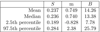
4.1 Posterior mean, medians and 95% credible intervals forS, mandB in Model (1.2.13). 103
4.2 Posterior median values for some parameters of interest for Models (1.2.13) and (2.1.4)
applied to the financial data. . . 105
4.3 Group sizes for the six groups of hospital firms based on ownership status and staff
ratio. . . 117
4.4 Posterior means, medians and 95% credible intervals for various parameters in Model
(4.2.3). . . 118
4.5 Posterior means, medians and 95% credible intervals for various parameters in Model
(4.2.2). . . 122
4.6 Posterior means, medians and 95% credible intervals for various parameters in Model
5.1 Maximum likelihood estimates of the NTS-binomial and beta-binomial models for the
first two simulated data sets. . . 156
5.2 Maximum likelihood estimates of the NTS-binomial and beta-binomial models for the
simulated data sets. . . 158
5.3 Maximum likelihood estimates for κ, µ, andα and the underlying values of these
parameters for the simulated data sets. . . 159
5.4 Maximum likelihood estimates and standard errors of the estimates for the
NTS-binomial and beta-NTS-binomial models for the six mice fetal mortality data sets. . . 162
5.5 Estimates of the first four central moments of the mixing distributions for the
beta-binomial and NTS-beta-binomial distributions for five mice fetal mortality data sets. . . . 163
5.6 AIC values for the competing models for each data set. The smallest value for each
data set is shown in bold and other AIC values are shown as differences from that
minimum. . . 164
5.7 BIC values for the competing models for each data set. The smallest value for each
data set is shown in bold and other BIC values are shown as differences from that
List of Figures
2.1 Kernel density estimate for the posterior of the weightεfor Model (2.1.4) for the first
simulated data set. . . 32
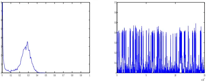
3.1 Kernel density estimate (left) and trace plot (right) for the posterior ofεfor the model
of M¨uller et al. (2004) for the first simulated data set. . . 59
3.2 Kernel density estimate (left) and trace plot (right) for the posterior of ε for Model
(2.1.4) for the first simulated data set. . . 60
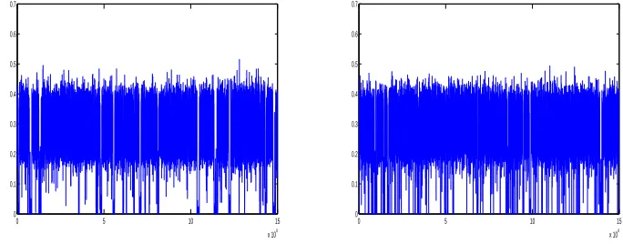
3.3 Trace plot for the posterior ofεwithout (left) and with the extra mix-split step (right)
for the model of M¨uller et al. (2004) for the first simulated data set. . . 67
3.4 Trace plot for the posterior ofεwithout (left) and with the extra mix-split step (right)
for Model (2.1.4) for the first simulated data set. . . 68
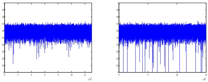
3.5 Trace plot for the posterior ofεwithout (left) and with the extra mix-split step (right)
for the model of M¨uller et al. (2004) for the second simulated data set. . . 68
3.6 Trace plot for the posterior ofεwithout (left) and with the extra mix-split step (right)
for Model (2.1.4) for the second simulated data set. . . 69
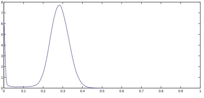
3.7 Kernel density estimate for the posterior ofεfor the model of M¨uller et al. (2004) for
the first simulated data set. . . 70
3.8 Predictive densities for the component distributions F1 (top), F2 (middle) and F0
(bottom) (left) and of F∗
1 (top) andF2∗ (bottom) (right) for the model of M¨uller et al. (2004) for the first simulated data set. . . 70
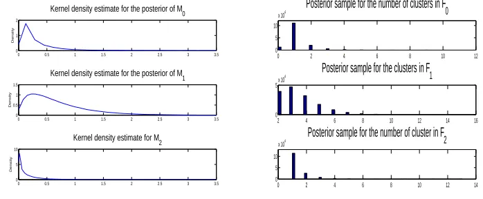
3.9 Posterior distributions ofM0, M1andM2(left) and posterior samples forK0, K1andK2
(right) for the model of M¨uller et al. (2004) for the first simulated data set. . . 71
3.10 Posterior distributions for S (top), m (middle) and B (bottom) for the model of
3.11 Kernel density estimate for the posterior ofεfor Model (2.1.4) for the first simulated
data set. . . 72
3.12 Predictive densities for the component distributions F1 (top), F2 (middle) and F0
(bottom) (left) and ofF∗
1 (top) andF2∗(bottom) (right) for the basic proposed model for the first simulated data set. . . 73
3.13 Posterior distributions ofM0(top) and M1(bottom) (left) and ofy(top) andx
(bot-tom) (right) for Model (2.1.4) for the first simulated data set. . . 73
3.14 Posterior distributions ofK0,K1andK2for Model (2.1.4) for the first simulated data
set. . . 74
3.15 Posterior distribution ofεfor the model of M¨uller et al. (2004) for the second simulated
data set. . . 75
3.16 Predictive densities for the component distributions F1 (top), F2 (middle) and F0
(bottom) (left) and of F∗
1 (top) andF2∗ (bottom) (right) for the model of M¨uller et al. (2004) for the second simulated data set. . . 76
3.17 Posterior distributions ofM0, M1andM2for the model of M¨uller et al. (2004) for the
second simulated data set. . . 79
3.18 Kernel density estimate for the posterior ofεfor Model (2.1.4) for the second simulated
data set. . . 79
3.19 Predictive densities for the component distributions F1 (top), F2 (middle) and F0
(bottom) (left) and of F∗
1 (top) andF2∗ (bottom) (right) for Model (2.1.4) for the second simulated data set. . . 80
3.20 Posterior distributions ofM0(top) and M1(bottom) (left) and ofy(top) andx
(bot-tom) (right) for Model (2.1.4) for the second simulated data set. . . 80
3.21 Posterior distribution ofεfor the model of M¨uller et al. (2004) for the third simulated
data set. . . 81
3.22 Predictive densities for the component distributions F1 (top), F2 (middle) and F0
(bottom) for the model of M¨uller et al. (2004) for the third simulated data set. . . . 82
3.23 Kernel density estimate for the posterior ofεfor Model (2.1.4) for the third simulated
data set. . . 82
3.24 Predictive densities for the component distributions F1 (top), F2 (middle) and F0
(bottom) for the basic proposed model for the third simulated data set. . . 83
3.25 Posterior distributions (left) and trace plots (right) forε1 (top),ε2 (bottom) for the
4.1 Trace plots forεin Model (1.2.13), with (right) and without (left) the mix-split step. 99
4.2 Posterior distribution ofε, Model (1.2.13). . . 99
4.3 Histograms of the data (left) and predictive densities forF∗
1 andF2∗ (right). . . 100 4.4 Predictive densities forF1 (top),F2 (middle) andF0 (bottom) for Model (1.2.13). . 101
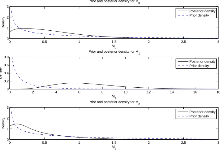
4.5 Prior (dashed line) and posterior (solid lines) distributions of M0, M1 andM2 in
Model (1.2.13). . . 102
4.6 Posterior distributions ofK0, K1andK2for the M¨uller et al. (2004) model. . . 103
4.7 Trace plots forεin Model (2.1.4) with (right) and without (left) the mix-split step. . 104
4.8 Posterior distribution ofεin Model (2.1.4). . . 104
4.9 Predictive densities forF1 (top),F2 (middle) andF0 (bottom) for Model (2.1.4). . . 105
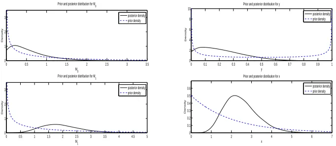
4.10 Prior (dashed line) and posterior (solid line) distributions of M0 (top), M1
(bot-tom)(left) andy (top),x(bottom)(right) in Model (2.1.4). . . 106
4.11 Posterior distributions ofK0 (top),K1 (middle) andK2 (bottom) in Model (2.1.4). . 107
4.12 Posterior distribution ofεfor Model (4.2.3) applied to the non-profit hospitals. . . . 119
4.13 Trace plots forε, with (right) and without (left) the mix-split step for Model (4.2.3)
applied to the non-profit hospitals. . . 119
4.14 Posterior distributions ofM0(top),M1(bottom)(left) andy (top),x(bottom)(right)
for Model (4.2.3) and the non-profit hospitals. . . 120
4.15 Predictive densities (left) and cumulative distributions (right) for the efficiency of
firms in the low staff ratio (solid line) and the high staff ratio group (dashed line) for
Model (4.2.3) applied to the non-profit hospitals. . . 120
4.16 Predictive densities for the efficiency of a firm in F1 (above), F2 (centre) and F0
(below) for Model (4.2.3) for the non-profit hospitals. . . 121
4.17 Quartile plots for the efficiencies of the firms in theF∗
1 (left) andF2∗(right) for Model (4.2.3) applied to the non-profit hospitals. . . 122
4.18 Posterior distribution ofεfor Model (4.2.2) for the non-profit hospitals. . . 123
4.19 Trace plot forεfor Model (4.2.2) for the non-profit hospitals. . . 124
4.20 Posterior distributions forM0, M1and M2for Model (4.2.2) for the non-profit hospitals.125
4.21 Predictive densities (left) and cumulative distributions (right) for the efficiency of
firms in the low staff ratio (solid line) and the high staff ratio group (dashed line) for
Model (4.2.2) applied to the non-profit hospitals. . . 126
4.22 Predictive densities for the efficiency of a firm in F1 (above), F2 (centre) and F0
(below) for Model (4.2.2) for the non-profit hospitals. . . 127
4.24 Trace plot forεfor Model (4.2.4) for the non-profit hospitals. . . 129
4.25 Posterior distributions ofM0(top),M1(bottom)(left) andy (top),x(bottom)(right)
for Model (4.2.4) for the non-profit hospitals. . . 129
4.26 Predictive densities (left) and cumulative distributions (right) for the efficiency of
firms in the low staff ratio (solid line) and the high staff ratio group (dashed line) for
Model (4.2.4) applied to the non-profit hospitals. . . 130
4.27 Predictive densities for the efficiency of a firm in F1 (above), F2 (centre) and F0
(below) for Model (4.2.4) for the non-profit hospitals. . . 131
4.28 Predictive densities for the efficiency of firms in the low staff ratio (solid line) and
the high staff ratio group (dashed line) for Models (4.2.3) (left) and (4.2.2) (right)
applied to the government hospitals. . . 131
4.29 Posterior distribution of the weight ε for Models (4.2.3) (left) and (4.2.2) (right)
applied to the government hospitals. . . 131
4.30 Posterior distribution (left) and trace plot (right) for ε for Model (4.2.4) for the
government hospitals. . . 132
4.31 Prior distribution ofεin Model (4.2.2) (left), (4.2.3) (middle) and (4.2.4) (right). . . 132
4.32 Predictive densities for the efficiency of firms in the low staff ratio (solid line) and the
high staff ratio group (dashed line) (left) and predictive densities forF1 (above),F2
(centre) andF0 (below) (right) for Model (4.2.4) applied to the government hospitals. 132
5.1 The Variance and kurtosis of NTS distribution with mean 0.5: (a) showsκversus the
variance, (b) showsκ versus the kurtosis and (c) shows variance versus kurtosis. In
each graph: S= 0.1 (solid line),S= 1 (dashed line) andS = 10 (dotted line). . . . 149
5.2 Skewness vs κfor various values of the mean for some MNTS distributions. In each
graph: S= 0.1 (solid line), S= 1 (dashed line) andS= 10 (dotted line). . . 149
5.3 Skewness vs variance and kurtosis vs skewness for some MNTS distributions. . . 150
5.4 Histogram ofpi used in the first two simulated data sets. . . 156
5.5 Kernel density estimates for the underlying pi in a NTS-binomial (top) and
beta-binomial model (bottom) for simulated data set 3. . . 160
5.6 Kernel density estimates for the underlying pi in a NTS-binomial (top) and
beta-binomial model (bottom) for simulated data set 11. . . 160
5.7 Kernel density estimates for the underlying pi in a NTS-binomial (top) and
5.8 Density estimates for the mixing distribution for the NTS-binomial (solid line) and
beta-binomial (dashed line) models evaluated at the maximum likelihood estimates
for the mice fetal mortality data. . . 163
5.9 Profile log-likelihoods for the parameters in the MNTS-binomial model for the HS1
Acknowledgments
I would first like to thank my two supervisors, Professor Mark F. J. Steel and Dr Jim E. Griffin.
Their support and guidance during the last four years has been invaluable.
I would also like to thank my two examiners, Professor Jim Q. Smith and Professor Peter M¨uller
for their suggestions in improving this work.
I am also very grateful to the members of the Department of Statistics of the University of Warwick
for providing a friendly, supporting and stimulating environment.
I feel more than obliged to thank my family. Without their continuous support, love and
encour-agement I would not have been able to make it to the end.
I would also like to deeply thank all my friends for their support and for making this journey much
more enjoyable.
Finally, I would like to thank the Centre for Research in Statistical Methodology (CRiSM), the
Engineering and Physical Sciences Research Council (EPSRC) and the Ministry of Finance of the
Declarations
I declare that the contents of this thesis are based on my own research in accordance with the
regulations of the University of Warwick. The work in this thesis is original, unless where indicated
Abstract
Bayesian nonparametric modelling has recently attracted a lot of attention, mainly due to the
ad-vancement of various simulation techniques, and especially Monte Carlo Markov Chain (MCMC)
methods. In this thesis I propose some Bayesian nonparametric models for grouped data, which
make use of dependent random probability measures. These probability measures are constructed
by normalising infinitely divisible probability measures and exhibit nice theoretical properties.
Im-plementation of these models is also easy, using mainly MCMC methods. An additional step in
these algorithms is also proposed, in order to improve mixing. The proposed models are applied
on both simulated and real-life data and the posterior inference for the parameters of interest are
investigated, as well as the effect of the corresponding simulation algorithms. A new,n-dimensional
distribution on the unit simplex, that contains many known distributions as special cases, is also
proposed. The univariate version of this distribution is used as the underlying distribution for
mod-elling binomial probabilities. Using simulated and real data, it is shown that this proposed model is
Abbreviations
AIC Akaike information criterion
BB beta-binomial
BIC Bayesian information criterion
cdf cumulative distribution function
DP Dirichlet process
EPPF exchangeable product partition formula
iff if and only if
MC Monte Carlo
MCMC Monte Carlo Markov chain
MDP mixture of Dirichlet processes
MH Metropolis-Hastings
MLE maximum likelihood estimate
N-IGP normalised inverse-Gaussian process
NRM normalised random measure
pdf probability distribution function
PDP product of Dirichlet processes
RJMCMC reversible jump MCMC
RPM random probability measure
RWMH random walk Metropolis-Hastings
SF stochastic frontier
Notation
The following notation is used throughout this thesis, unless otherwise stated. We usually use normal
font type for scalars andboldfont type for vectors, unless otherwise stated.
IN The set of natural numbers
IR The set of real numbers
∅ The null set
δx Dirac measure
Bc The compliment set of a setB |x| The absolute value of a numberx
d
= Equality in distribution, i.e. identically distributed
A−1 The inverse of a matrixA
Chapter 1
Introduction
Bayesian nonparametric modelling has recently attracted a lot of attention, partly because of the
advancement of simulation methods, and especially Monte Carlo Markov chain (MCMC) methods.
These models offer a flexible prior specification of the distribution of some data and can therefore
be particularly useful in cases where it is preferred not to impose much prior structure on the
distribution of those data. Bayesian nonparametric models can also be used in a variety of ways in
modelling two or more correlated data sets (for example spatial data).
1.1
Bayesian Nonparametric Modelling
The term “Bayesian nonparametric model” refers to a probability model with infinitely many
pa-rameters (Bernardo and Smith, 1994), which results in inference which is directly comparable to
classical nonparametric models. These methods have attracted a lot of attention recently, especially
because of the recent advances in some simulation techniques, and especially Monte Carlo Markov
chain methods, which facilitate the simulation of the posterior distributions of the parameters of
interest. These models can be particularly useful in cases when there is uncertainty about the
un-derlying distribution of some data, so modelling this distribution in a flexible way is desirable. As
a result, they can be naturally applied to density estimation and regression models.
There are many classes of Bayesian nonparametric models. For the density estimation problem,
i.e. the problem of estimating the underlying distribution(s) of some data, it is assumed that the
data, say Y1, Y2, . . . , Yn, come from a distribution F or, more generally, each Yi ∼ Fi. In the
Bayesian nonparametric setting, one considers these distributions also as random and assigns prior
by Pitman (1996), P´olya trees (introduced by Ferguson (1974) and developed by Lavine (1992,
1994)), Bernstein polynomials and the very general class of Random Probability Measures (RPMs
- see e.g. Crauel (2002)). We also note an interesting and very rich subclass of the RPM, the
normalised random measures, which will be described in Section 1.2.3. For the regression problem
yi =g(xi) +ǫi, i = 1,2, . . . , n(where the bold symbols denote vectors), many approaches include
some collection of distributions, say B = {f1, f2, . . .}, and write g = P∞k=1bkfk, for some basis
coefficients b1, b2, . . .. Popular choices for this collection B include spline, Fourier and wavelet
models. For a more detailed review of the aforementioned (and more) Bayesian nonparametric
methods, see M¨uller and Quintana (2004).
At this point something more about the RPMs needs to be said, since they are not only a very
rich class of models, but also the one mostly used in practise. As the name indicates, a RPM is a
probability measure that is itself taken to be random. Alternatively, as stated in Ferguson (1974),
it can be thought of as a random variable whose values are probability measures. A more formal
definition is the following:
Definition 1. Let X be a Polish space and B denote its σ−algebra. Let also (Ω,F,P) denote a probability space. A map
µ : B ×Ω →[0,1]
(B, ω) →µω(B)
satisfying
1. ∀ B∈ B, µω(B)(as a function of ω) is measurable,
2. for P-almost everyω∈Ω,µω(B) (as a function ofB) is a Borel probability measure
is said to be a random probability measure on X.
Within the Bayesian framework, a prior distribution is assigned to a RPM (i.e. a prior distribution
of the random distribution). The most widely used prior specification for this random probability
measure in the literature is the Dirichlet process (DP), introduced by Ferguson (1973). Other
choices include the normalised inverse-Gaussian process (N-IGP) advocated by Lijoi et al. (2005),
the invariant DP (Dalal, 1979) and the aforementioned P´olya trees.
Finally, note that these random measures fit naturally in a standard hierarchical model, for
example:
Yi∼f(Yi;θi), i= 1,2, . . . , n
G∼RPM(ψ)
ψ∼h(ψ).
This setup can be useful in cases where the realisations of the RPM used are discrete distributions,
whereas the data under consideration are continuous. This will be demonstrated using the DP as
the underlying RPM in the next subsection.
1.1.1
The Dirichlet process
First, the Dirichlet (Dir) distribution is defined:
Definition 2. Ann-dimensional random variableX = (X1, X2, . . . , Xn)defined on the unit simplex
is said to follow a Dirichlet distribution with parametersa1, a2, . . . , an+1>0, denoted Dir(a1, a2, . . . , an+1), if its density with respect to the Lebesque measure is:
fX(x) =
Γ(a1+a2+· · ·+an+1)
Γ(a1)Γ(a2)· · ·Γ(an+1) n
Y
i=1
xai−1
i (1− n
X
j=1
xj)an+1−1, x1, x2, . . . , xn≥0,
n
X
k=1
xk≤1.
In the above definition Γ denotes the gamma function, Γ(x) = R0∞tx−1e−tdt. Notice that the
univariate Dirichlet distribution is the known beta (Be) distribution:
Definition 3. A random variable X defined on [0,1] is said to follow a beta distribution with parameters a1 ≥0 anda2 ≥ 0, a1+a2 > 0, denoted Be(a1, a2), if its density with respect to the Lebesque measure is:
fX(x) = Γ(a1+a2)
Γ(a1)Γ(a2)x
a1−1(1
−x)a2−1, 0≤x≤1.
Ifa1= 0, thenX = 0 almost surely and ifa2= 0, X = 1almost surely.
A simple definition of the Dirichlet process is then the following:
Definition 4. A random probability functionF is said to follow a Dirichlet process with parameters M andH0 if for any partition (A1, A2, . . . , Ak) of the probability space Ω, such that all Ai ∈ F,
theσ−algebra ofΩ,the vector of random probabilities(F(A1), F(A2), . . . , F(Ak))follows a Dirichlet
distribution with parametersM H0(A1), M H0(A2), . . . , M H0(Ak).
Symbolically:
F ∼DP(M, H0)def⇔ ∀ partition (A1, A2, . . . , Ak) of Ω, A1, A2, . . . , Ak ∈ F
As shown in Lemma 1 of Ferguson (1973), the existence of such a process is verified by showing that
the Kolmogorov consistency conditions hold.
As seen from the definition, there are two parameters characterizing the DP:H0 andM.
H0 is a distribution function and is called the base or centering distribution of the DP. It can be
seen as the centre of the process, since
∀B∈ F, E (F(B)) =H0(B). (1.1.1)
The parameterM >0 is a scalar called the concentration or precision parameter of the process, and
it controls the variability of the process aroundH0, since
∀ B∈ F,Var (F(B)) = H0(B) (1−H0(B))
1 +M . (1.1.2)
So, intuitively,M can also be seen as a measure of our belief in the base distributionH0.
In fact, in his seminal paper, Ferguson (1973) uses a non-null finite measureαas the parameter of
the DP. Then, by considering the parametrisationM =α(Ω) andH0= α(Ω)α , we get the definition above and a better understanding of the role played by this measureα.
The reason for the popularity of the Dirichlet process is its mathematical properties, which lead to
algebraic and computationally convenient expressions, therefore allowing for relatively easy posterior
inference when combined with MCMC techniques. These properties include simple expressions for
the expectation and variance of its realisations, as seen in (1.1.1) and (1.1.2).
The DP can also be represented using a stick-breaking representation (Sethuraman and Tiwari,
1982; Sethuraman, 1994): IfF ∼DP(M, H0),then
F(·) =
∞
X
i=1
wiδθ∗
i(·), whereθ
∗
i iid
∼ H0, wi=Vi
Y
j<i
(1−Vj), whereViiid∼Be(1, M) (1.1.3)
whereδx denotes the Dirac measure giving mass 1 to the valuex.
As can be seen from (1.1.3), any realisation of the DP is, with probability 1, a discrete distribution.
This is an obvious drawback when one wants to model data from continuous distributions. On the
other hand, this discreteness allows for clustering the values of a random distribution following a
DP:
LetF ∼DP(M, H0),whereH0is a continuous distribution and assume a sampleθ1, θ2, . . . , θnfrom
F. The number of discrete θi (denoted by θ∗i), will be K ≤n. The distribution of K is given in
Escobar and West (1995):
P(K=k|M, n) =cn(k)n!Mk
Γ(M)
Γ(M +n), k= 1,2, . . . , n (1.1.4)
wherecn(k) =P(K=k|M = 1, n),not involvingM.
If, on the other hand, H0 was discrete, we would again have discrete values, but now there is the
possibility that some of the clusters created by the discreteness of the DP (not of H0) would be
located at the same values.
Notice also that, as (1.1.4) suggests, for higher values of the concentration parameter, higher
probabilities are given to larger number of clusters. The intuition for this is that higher values of
M indicate less variation from the base distribution H0, i.e. more belief in H0. As a result, more
observations from the DP will actually be taken from this base distribution. The above observations
are consistent with (and complemented by) equation (1.1.5) below.
Next, the P´olya-urn representation of the DP are presented, i.e. an expression of the possible
allocations of a new observation from the DP, given previous observations from the same DP. This
representation was noted by Blackwell and MacQueen (1973) and has also a simple form: having
observedθ1, θ2, . . . , θn fromF ∼DP(M, H0),the (posterior) distribution of a new observationθn+1 is as follows:
∀ A∈ F, P(θn+1∈A|θ1, θ2, . . . , θn) =
M
M+nH0(A) +
1
M+n
n
X
i=1
δθi(A). (1.1.5)
This means that any new value will be set equal to one of the previous valuesθi (with probability
1
M+n for eachθi) or will be a new draw from the base distribution (with probability M
M+n). Again,
notice that for higher values ofM, more clusters are expected to be created for a specific data size.
A similar expression to the P´olya-urn representation is the so-called Chinese restaurant
repre-sentation (Aldous, 1985; Pitman, 1996). Before explaining this algorithm, let us define the indicator
functionssi, i= 1,2, . . . , n, such that
si=j⇔θi≡θj∗, j= 1,2, . . . , K,
where (θ1, θ2. . . , θn) is a sample from a DP(M, H0)-distributed random distribution F and (θ∗1, θ∗2, . . . , θK∗)
is the vector of discrete values (clusters) of these data.
The Chinese restaurant representation now gives the probabilities of all possible values of a new
indicatorsn+1, corresponding to a new observation from F|θ1, θ2, . . . , θn.It is clear thatsn+1 takes values in the set{1,2, . . . , K+ 1}, where the firstKvalues correspond to the already existing clusters and the last value corresponds to a new cluster being created. These probabilities are as follows:
P(sn+1=j) =
nj
n+M , j= 1,2, . . . , K
M
n+M , j=K+ 1,
Using the P´olya-urn scheme for a single DP with parameterM, it is easy to derive the
Ex-changeable Product Partition Formula (EPPF) for this model:
p(s|M) =Mk Γ(M)
Γ(M +n)
K
Y
i=1
Γ(ni) (1.1.6)
wheres= (s1, s2, . . . , sn) is the vector of all allocation parameters.
Finally, the property that, in fact, characterizes the DP, is its conjugacy: givenθ1, θ2, . . . , θn
from F ∼DP(M, H0), the posterior distribution ofF is again a DP with parametersM +nand
H0+Pni=1δθi:
F|θ1, θ2, . . . , θn∼DP M+n, H0+
n
X
i=1
δθi
!
.
Apart from its obvious advantages stated above, there is the quite unpleasant feature of the
DP that its realisations are always discrete distributions. As a result, modelling continuous data
using the DP as the distribution of their distribution would be inappropriate.
The usual solution to this problem is to add an additional level in the model, by assuming that
the data come from a continuous distribution with parameters θ and set the distribution of the parametersθ to follow a DP (Ferguson, 1983; Lo, 1984):
Yi∼f(Yi;θi,ζ), i= 1,2, . . . , n
θi iid
∼G
G∼DP (M, H0(ψ)) (1.1.7)
M ∼h1(M), ζ∼h2(ζ), ψ∼h3(ψ)
where ζ are any other parameters in the likelihood f not modeled using the DP and ψ are the parameters of the base distributions (if any).
This setup is referred to as mixture of Dirichlet process (MDP) model, and was introduced by
Antoniak (1974). Note also that the distribution of eachYi (givenζ) is given by convolvingf with
G∼DP:
f(Yi;ζ) =
Z
f(Yi;θ,ζ)dG(θi), whereG∼DP(M, H0(ψ))
and this, together with the discrete nature of the realisations of the DP, will lead to a mixture model
forYi (givenζ) (Antoniak, 1974).
1.1.2
Computational issues
For models with many parameters, the joint posterior distribution of all parameters is usually
fall in this category. Therefore, most inference using these models involves advanced computational
methods, and mostly Monte Carlo Markov Chain (MCMC) methods are used. Other simulation
methods are also applicable, like sequential importance sampling (see, for example, MacEachern
et al., 1999; Fearnhead, 2004) and variational inference methods (Beal and Ghahramani, 2003).
MCMC methods consist of constructing a Markov Chain (i.e. a chain where each updating
step depends only on the previous iteration of the chain) that has the desired posterior distribution
of all parameters in the model as its stationary distribution.
The mostly used MCMC method is the Gibbs sampling. According to this method, we start
with some initial values for our parameters. Then, in each step of the chain, each parameter in
the model is sequentially simulated from its full conditional distribution, i.e. the distribution of
the specific parameter given the data and all the other parameters. In each case the values of
the parameters of interest are recorded and at the end some initial part of the chain is discarded
as burn-in. The rest of the output consists of samples from the joint posterior distribution of all
parameters. From this output the values of a specific parameter can also be taken, and those
values will be samples from the posterior distribution of this parameter. In this method, if a full
conditional distribution is of known form, for example if it is a beta distribution, simulating from it
is straightforward. If, on the other hand, simulating from a full conditional distribution directly is
not possible, Metropolis-Hastings (MH) steps or slice sampling can be used instead.
MH updating steps consist of proposing a value for the parameter that is to be updated and
calculating the acceptance probability of the proposed value. This acceptance probability takes into
account both the full conditional distribution of the parameter and the probability of the transition
from the existing value of the parameter to the one proposed. More specifically, the acceptance
probabilityαfor moving a parameterϑfrom its current valueϑ0 to a new valueϑ′ is:
α(ϑ0, ϑ′) = min
1, f(ϑ′)
f(ϑ0)
q(ϑ′, ϑ0)
q(ϑ0, ϑ′)
.
wheref is the full conditional distribution ofϑandq(a, b) is the transition probability from a value
ato a value b, and depends on the method of proposing these new values. Then, with probability
α(ϑ0, ϑ′), the value ofϑis changed toϑ′, otherwise it remains unchanged: ϑ=ϑ0.
Popular choices for proposing new values in a MH step include independence MH steps (when
the proposed value is taken independently of the current value) and the random walk
Metropolis-Hastings steps (RWMH), when the proposed value is the sum of the existing value and a value from
a zero-mean random variate. Roberts and Rosenthal (2001) discuss monitoring of RWMH updating
steps, in order to optimise mixing. In the following, RWMH steps will mostly be used when the full
Slice sampling is a parameter augmentation technique, in which the parametric space is
ex-tended to include some auxiliary variables (see, for example, Damien et al., 1999; Neal, 2003).
Sup-pose that we want to sample from a distributionf(x). If this distribution is difficult to sample from,
we can extendf(x) tog(x, u), whereuis an auxiliary variable andgis such thatRg(x, u)du=f(x)
andg(u|x) = R g(u,x)
g(x,u)du is a uniform distribution on a set (and therefore easy to sample from, for
example, using inverse transformation methods). The joint densitygis also chosen such thatg(x|u) is also easy to sample from. We can then iteratively sample fromg(x|u) and g(u|x), and the value ofxobtained will be a draw fromf(x). As a simple example, considerf(x) =xe−x2. We can then
setg(x, u)∝x1(0<u<e−x2
), where the indicator function 1( ) takes the value 1 if the expression in the subscript is true, and 0 otherwise. Theng(u|x) is the uniform distribution in0, e−x2
, whereas
g(x|u) =x1(|x|<−log(u)), and therefore easy to sample from.
Since the MDP Model (1.1.7) is the one mostly used in Bayesian nonparametric inference, it
would be useful to present the basic methods of implementation using MCMC methods. This will
also provide a first introductory insight to the algorithms that will be presented in the next sections,
since more or less the same principles apply. For simplicity, it is assumed that eachθi is scalar,
there are no extra parametersζin the likelihood and the parameters of the base distributionψ are fixed. Usually, in the more general case where additional parameters are introduced in the model,
their full conditional distributions are explicitly known and easy to sample from.
As mentioned before, due to the infinite number of point masses and weights of any realisation of
the Dirichlet process (as seen by the stick-breaking representation), it is impossible to simulate from
the DP directly. However, in cases where one is not directly interested in the unknown random
distribution itself, but rather in the posterior distributions of some parameters of the model (which
is very common in practice), a sample from those posterior distributions can be obtained using
MCMC methods. It is also possible to get samples from the predictive distribution of a parameter
whose distribution is DP-distributed.
There are two main approaches in simulating Model (1.1.7). One approach is to use marginal
methods, which consist of integrating the unknown distribution out of the posterior distributions
and using the P´olya-urn representation of the Dirichlet process. The second approach is to use
conditional methods, which consider the DP as part of the MCMC algorithm.
Marginal methods
This is the method mostly used in the literature. Usually this algorithm uses a Gibbs sampler,
especially when the likelihoodf(Y;θ) and the base distribution H0(θ) form a conjugate pair for θ
algorithms concerning the marginal method are based on the seminal paper of Escobar and West
(1995), which is itself based on the work of Escobar (1988, 1994). Very good descriptions of some
marginal algorithms can be found in Escobar and West (1998) and MacEachern (1998).
In order to implement the Gibbs algorithm, the full conditional distributions of all
parame-ters in the model, i.e. the distributions of each parameter given all the other parameparame-ters and the
dataY1, Y2, . . . , Yn, need to be calculated. The conditional independence relationships between the
parameters that the hierarchical structure of this model expresses also enhance these calculations.
Regarding the full conditional distribution of eachθi, the P´olya-urn representation of the DP (1.1.5)
can be used in order to integrate out the unknown distribution. The exchangeability ofθi in this
expression leads to the following posterior distribution forθi:
p(θi|θ−i,Y, M,ψ) =q0
f(Yi|θi)h0(θi|ψ)
R
f(Yi|θi)dH0(θi|ψ)
+X
j6=i
qjδθj(θi) (1.1.8)
where h0(θi|ψ) = dH0dθ(θii|ψ) is the pdf of H0, Y is the data set, θ−i = (θ1, . . . , θi−1, θi+1, . . . , θn),
q0∝M
R
f(Yi|θi)dH0(θi|ψ), qj ∝f(Yi|θj) and the factors of proportionalities are the same for each
weight and such that the weights add to 1. This structure indicates how easy it is to simulate each
θi given all the others. What is needed is to calculate the weightsq0 andqj, j6=iand then assign
θito one of the otherθj with probabilitiesqj, j6=i, or draw a new value from the base distribution
H0, with probabilityq0. The tricky part is calculating the integral appearing in the expression for
q0. On the other hand, when the base distribution H0 and the likelihoodf form a conjugate pair,
this integral will be trivial.
As far as the precision parameterM is concerned, it was demonstrated in Escobar and West
(1995) that it is better to consider it as a random variable and impute it in the MCMC algorithm.
In the same article, the authors give a Ga(α, β) prior distribution toM and propose a very simple
way to update this quantity, using a fine algebraic trick.
Definition 5. A random variable X is said to follow a gamma distribution with parameters α >
0andβ >0, denoted by Ga(α, β), if its density with respect to the Lebesque measure is:
fX(x) =
β−α
Γ(α)x
α−1e−x/β, x >0.
The full conditional distribution ofM in the specific model is proportional to its prior and to the
dis-tribution of the number of cluster,K, shown in (1.1.4). Therefore,f(M| · · ·)∝Mα+K−1e−M/β Γ(M) Γ(M+n) and the last fraction can be substituted using the formula
Γ(M) Γ(M+n) =
(M +n)B(M + 1, n)
whereB(a, b) =R01xa−1(1
−x)b−1dxis the usual beta function. This leads to:
f(M| · · ·) ∝ Mα+K−1e−M/β(M +n)B(M + 1, n) M
= Mα+K−2e−M/β(M +n)
Z 1
0
xM(1
−x)n−1dx.
The last expression can now be seen as the marginal distribution of the joint distribution ofM and
an auxiliary variable in (0,1), say ξ, where f(M, ξ| · · ·) ∝ Mα+K−2e−M/β(M +n)ξM(1
−ξ)n−1. The full conditionals of each of those quantities are as follows:
f(M|ξ,· · ·) ∝ Mα+K−2e−M(1/β−log(ξ))(M +n)
= Mα+K−1e−M(1/β−log(ξ))+nMα+K−2e−M(1/β−log(ξ))(M+n).
(i.e a mixture of gamma distributions), and
f(ξ|M,· · ·)≡Be(M + 1, n).
What one needs to do in order to simulate from M in each step in the MCMC algorithm is to
simulate from bothf(ξ|M,· · ·) and f(M|ξ,· · ·) sequentially. Each value ofξcan be discarded after
M is simulated, as it is just an auxiliary variable, whereas the values ofM will be kept and used in
the rest of the algorithm and in posterior inference.
Finally, it is also straightforward to include an additional step in the MCMC algorithm that
approximates the predictive distributionp(Yn+1|Y1, Y2, . . . , Yn) :
p(Yn+1|Y1, Y2, . . . , Yn) =
Z Z
· · ·
Z
p(Yn+1, θ1, θ2, . . . , θn|Y1, Y2, . . . , Yn)dθ1dθ2. . . dθn
=
Z Z
· · ·
Z
p(Yn+1|θ1, . . . , θn, Y1, . . . , Yn)f(θ1, . . . , θn|Y1, . . . , Yn)dθ1. . . dθn
=
Z Z
· · ·
Z
p(Yn+1|θ1, θ2, . . . , θn)f(θ1, θ2, . . . , θn|Y1, Y2, . . . , Yn)dθ1dθ2. . . dθn.
In words, the predictive distribution can be expressed as an expectation of the random vector
(θ1, . . . , θn) from its posterior distribution. This expression is very complicated to calculate
analyti-cally. On the other hand, this expectation can be approximated using Monte Carlo (MC) methods:
in each step of the MCMC algorithm after the burn-in period, a sample from theseθi’s is obtained.
These samples are actually samples from the posterior distribution of (θ1, . . . , θn). So, in each step
p(Yn+1|θt1, θ2t, . . . , θnt) (which will be a simple mixture distribution) is calculated, where the values
for the θt
expressions over all the MCMC cycles after burn-in, we get an approximation of the predictive
distribution.
An improvement to this algorithm was proposed by MacEachern (1994) and is almost always
used in this type of models, as it is easy to implement and improves the mixing of the chain. It
exploits the clustering of the values of a sample from a random distribution following a DP, as
mentioned before. Instead of using the actual values (θ1, θ2, . . . , θn), it uses the
reparametrisa-tion (θ∗
1, θ∗2, . . . , θK∗, s1, s2, . . . , sn), where the quantities are as defined before. The reason for this
reparametrisation is that now the discrete valuesθ∗
j are also updated, resulting in better mixing of
the Markov chain. Note that the prior distribution of theθ∗
j’s is the base distributionH0, so the full
conditional distribution for eachθ∗
i will be proportional to the product ofH0and of the product of the likelihood of the data that are associated with it,H0(θ∗
i)
Q
j:sj=ip(Yj;θ
∗
i). As for the updating
of the indicators, this will be the same as (1.1.8), withsreplacingθ.
Apart from the above method of improving the calculations, other tricks have been proposed
(see e.g. MacEachern (1998)). Some of them are:
1. Collapsing of the state space: The idea here is that, since we use simulation to avoid
dif-ficult integrals, one should try to evaluate as many integrals as possible before starting the
simulation. So, if possible, we integrate out some parameters from our model before the
simulations.
2. Blocking: The basic idea is to update parameters that are a posteriori highly correlated
together, and therefore improve the mixing of the chain.
3. Rao-Blackwellization: Proposed by Gelfand and Smith (1990), this technique suggests
replac-ing values generated as part of the simulation with appropriate conditional expectations. In
this way, one can benefit from conditional distributions, if they are of known form.
The nonconjugate case
This is the case where the likelihoodf and the base distributionH0 do not form a conjugate pair.
As a result, calculations of some integrals become nontrivial. For example, in the update ofθi (or
of thesi), we have the integral
R
f(y;θi)dH0(θi). Iff andH0 are not conjugate, calculating these integrals can be very difficult or even impossible. Although in nonparametric models a variety of
base distributions can be used, since these models are quite flexible and will adapt to the specific
choice (for example, a DP prior with M small can be used), there are cases where it seems more
discussed, among others, in West et al. (1994), MacEachern and M¨uller (1998), Neal (2000) and
Jain and Neal (2005) (all in the case of the MDP model).
The first paper provides the first algorithm designed for the nonconjugate case. The authors
here propose an MCMC scheme for simulating from the posterior distributions of the parameters in
the model. Their solution to the problematic integralR f(Yi|θi)dH0(θi) is to approximate it using
Monte Carlo approximation or, in the special case where only one of these MC samples is used, to
replace it byf(Yi|θ′),whereθ′ is a draw fromH0. However, as MacEachern and M¨uller (1998) note,
this approximation fails theoretically, as the resulting Markov chain might converge to a stationary
distribution that is not the same as the posterior distribution. Another issue about this method
is that it is not easy to evaluate the accuracy of the approximation, as this approximation occurs
within acceptance probabilities.
In the second reference the authors propose the so-called “no gaps algorithm”. This method
consists of augmenting the vector of discrete values (θ∗
1, θ∗2, . . . , θ∗K) to (θ∗1, θ∗2, . . . , θK∗, θ∗K+1, . . . , θ∗n).
The name of this method comes from the fact that the firstK values of the full vector of theθ∗
i’s
correspond to those clusters that are associated with at least one observation. As a result, there are
no gaps in the values of the indicatorssi, i= 1,2, . . . , n. Using this augmentation, the problematic
integral disappears and it is replaced by simple likelihood evaluations, since now all the new clusters
that might be used are associated with some value (θ∗
K+1 toθ∗n).
In Neal (2000), two methods are proposed. The first one involves MH proposals for the update
of the allocations si, i= 1,2, . . . , n, whereas the second method is very similar to the “no gaps”
algorithm of MacEachern and M¨uller (1998), but slightly more general.
Finally, in the last approach, Jain and Neal (2005) propose an MCMC algorithm, which in each
iteration proposes mix or split steps. More specifically, each mixing proposal consists of merging
two clusters of discrete values ofθinto one, and each splitting proposal suggests splitting one cluster
ofθ∗ into two separate ones. This algorithm is computationally expensive, but with good mixing
properties and can be a good choice in the nonconjugate case, if the other approaches fail to reach
equilibrium in a sensible amount of time.
Conditional methods
Conditional methods can be particularly useful when it is not easy to integrate the random
proba-bility measure out of the joint posterior distribution of all parameters in a model. The basic idea in
these methods is to impute the RPM in the parameter space and update it in the MCMC algorithm,
as well as the other parameters. However, this involves an infinite number of parameters, making
order to simulate from such a representation, an infinite number of weightswj and point massesθj∗
needs to be simulated. In practice, we need a finite version of this, and a suggested solution is using
some form of truncation, for example replacing the infinite sum in (1.1.3) withPNi=1wiδθ∗
i(·),forN
large enough (Ishwaran and Zarepour, 2000). Although the error produced by such approximations
can be controlled (Ishwaran and James, 2001), it would be preferable to avoid such approximations
completely. In the case of the DP as the distribution of the RPM, updates of the latter can be
per-formed using its stick-breaking representation (1.1.3). Papaspiliopoulos and Roberts (2008) show
that the approximation can be completely avoided, using a technique called retrospective sampling,
which will be demonstrated in the case of a DP-distributed RPM, as is the case for Model (1.1.7):
Suppose we want to create a sampleθ1, θ2, . . . , θn fromF ∼DP(M, H0). According to (1.1.3), if we
could create an infinite number of pairs (wj, θ∗j), we would then assign eachθi=θ∗j with probability
wj. This could be done usingUi∼U(0,1) and setting θi=θ∗j iff: j−1
X
k=0
wk< Ui≤
j
X
k=0
wk, (1.1.9)
wherew0 = 0. It is clear that, for a finite number of draws fromF, only a finite number of pairs
of weights and point masses is needed. Retrospective sampling method, now, simply exchanges the
order of simulation between the pairs (wj, θ∗j) and theUi’s: we create a finite number of these pairs,
and then check (1.1.9) for eachUi simulated. If for some of thoseUi’s, (1.1.9) is not satisfied, we go
back and simulate more of these pairs, until (1.1.9) is satisfied for somej.
Retrospective sampling for the simple MDP model:
By replacing the DP by its equivalent expression (1.1.3), the MDP model can be written as follows:
Yi∼f(Yi;θs∗i,ζ), i= 1,2, . . . , n
si∼
∞
X
j=1
wjδj, wherewj=Vj
Y
k<j
(1−Vk), whereViiid∼Be(1, M)
θ∗j ∼H0(ψ) (1.1.10)
M ∼h1(M), ζ∼h2(ζ), ψ∼h3(ψ).
As in the marginal method, it is assumed that we do not have any additional parametersζ in the likelihood and the parametersψ are fixed.
As mentioned above, since we just need a finite number ofθi≡θs∗i, only a finite number of weights
and point masses is needed. So, we start with a large number of them, and if at some point in the
simulation more are needed, we create them retrospectively. Another issue in this algorithm is that,
P∞
j=1wjf(Yi;θj∗) appears as a normalising constant. As a result, we cannot simulate from these
distributions directly. Papaspiliopoulos and Roberts (2008) propose a MH updating step in order
to overcome this problem. To sum up, the proposed iterative steps in the MCMC algorithm (given
an initial allocations= (s1, s2, . . . , sn) and settingN = max{s}) are the following:
1. Simulateθ∗
j, j= 1,2, . . . , N from their full conditional distributions.
2. SimulateVj, j= 1,2, . . . , N from their full conditional distributions and calculate the weights
wj =VjQm<j(1−Vm), j= 1,2, . . . , N.
3. Fori= 1,2, . . . , n,simulateUi∼U(0,1).
(a) Check if (1.1.9) is satisfied for some j ≤N. If yes, propose to update si using a MH
update. If this proposed step is accepted, perform the change, otherwise keep the same
value forsi.
(b) If, on the other hand, (1.1.9) is not satisfied for anyj ≤N, simulate a pair (VN+1, θN∗+1) from its prior distribution. CalculatewN+1=VN+1Qm≤N(1−Vm), setN =N+ 1 and
go Step (3a).
4. SetN = max{s}.
5. Update M from its full conditional distribution, having first marginalised over the pairs
(wj, θ∗j) not associated with any observation.
The above full conditional distributions are simple expressions and can be seen in Proposition 1 of
Papaspiliopoulos and Roberts (2008). Notice also that, without the marginalisation mentioned in
the update ofM, one will not be able to perform this step, as the number of unused pairs is infinite.
Another method of overcoming the infinite number of parameters appearing in the
stick-breaking representation of some RPMs (for example, those following a DP) without confronting to
any approximation is the slice sampler, as demonstrated in Walker (2007). Consider, for example,
Model (1.1.10), with the same simplifications mentioned above. Using (1.1.3), it is straightforward
to see that the conditional likelihood of each dataYi will be
f(Yi|w,θ∗) =
∞
X
j=1
wjf(Yi;θ∗j). (1.1.11)
By introducing a latent parameterui, (1.1.11) can be written as:
f(Yi, ui|w,θ∗) =
∞
X
j=1
1(ui<wj)f(Yi;θ∗j). (1.1.12)
By integrating outui we get (1.1.11), whereas this expression can be used to derive the full
with observationYi), when those parameters are embedded at the parametric space of our model.
On the other hand, given theseui’s, the model will now have only a finite number of parameters,
therefore allowing for exact simulation from their full conditional distributions. As for the unused
pairs of (wj, θj∗), they need not be considered in the MCMC algorithm, as they can be integrated
out. More details are given in Walker (2007).
1.1.3
The normalised inverse-Gaussian process
The normalised inverse-Gaussian process (N-IGP) seems to be a very good alternative to the Dirichlet
process. It was introduced by Lijoi et al. (2005), similarly to the way Ferguson (1973) introduces the
DP. One possible definition makes use of the normalised inverse-Gaussian distribution in the same
way the Dirichlet distribution is used in the DP:
Definition 6. A random variable X is said to have the inverse-Gaussian distribution with shape parameterα≥0 and scale parameter γ > 0, symbolically X ∼IG(α, γ), if its density with respect to the Lebesque measure is the following:
fX(x) =
α
√
2πx
−3/2exp
−12
α2
x +γ
2x
+γα
, x≥0, for α >0
andX= 0 almost surely forα= 0.
In the following assume, without loss of generality, thatγ= 1 (since it is a scale parameter).
Definition 7. Let X1, X2, . . . , Xn be independent random variables with Xi ∼ IG(αi,1), i =
1,2, . . . , n, with allαi >0.Then, the random vectorW = (W1, W2, . . . , Wn), whereWi=PnXi
j=1Xj, i=
1,2, . . . , nis said to follow a normalised inverse-Gaussian distribution with parametersα1, α2, . . . , αn.
Symbolically,W ∼N-IG(α1, α2, . . . , αn).
Another way to define the N-IG distribution is using the derived probability density function. More
specifically, ifW = (W1, W2, . . . , Wn)∼N-IG (α1, α2, . . . , αn), its pdf will be:
fW(w) =
ePni=1αiQn
i=1αi
2n/2−1πn/2 K−n/2
p
An(w1, . . . , wn) w31/2w
3/2
2 · · ·wn3/2[An(w1, . . . , wn)]n/4
−1
where An(w1, . . . , wn) =Pni=1α 2
i
wi andKdenotes the modified Bessel function of the third type.
Definition 8. A random probability measureF is said to follow a normalised inverse-Gaussian pro-cess with parametersM andH0if for any partition(A1, A2, . . . , Ak)of the probability spaceΩ, such
follows a normalised inverse-Gaussian distribution with parametersM H0(A1), M H0(A2), . . . , M H0(Ak).
Symbolically:
F∼N-IGP(M, H0)def⇔ ∀ partition (A1, A2, . . . , Ak) of Ω, A1, A2, . . . , Ak∈ F,
(F(A1), F(A2), . . . , F(Ak))∼N-IG(M H0(A1), M H0(A2), . . . , M H0(Ak)).
In the original definition of Lijoi et al. (2005), instead ofM and H0 there is only a nun-null finite
measureα. ForM =α(Ω)>0 andH0(·) = αα(Ω)(·), we can see that this is just a reparametrisation. In the same article, the authors use Proposition 3.9.2 of Regazzini (2001), in order to show that the
N-IGP is well defined.
The N-IGP has many similarities with the DP. The first obvious one is the parametrisation.
Again, there is a distribution,H0 and a positive scalar,M, and by studying the expressions of the
expectation and variance of any realisation of the N-IGP, one will see that those two parameters
have the same intuitive interpretation as the corresponding parameters of the DP. More specifically,
ifF ∼N-IGP(M, H0), we have:
∀ B∈ F, E (F(B)) =H0(B) and Var (F(B)) =H0(B) (1−H0(B))M2eMΓ( −2, M) where Γ(a, x) =Rx∞e−tta−1dtis the incomplete gamma function. As before,H
0 can be seen as the
centre of the process andM as a measure of our belief in this centre. Another common property of
the N-IGP and the DP is the almost sure discreteness of their realisations. This can be a problem
when modelling continuous data, but again this can be resolved using mixtures of N-IG processes,
as in the case of MDPs.
It is also worth mentioning that the N-IGP and the DP are the only known processes whose finite
dimensional distributions are known explicitly.
The P´olya-urn representation of the N-IGP is also known. The structure is similar to the
expression for the DP, with more complicated expressions for the weights:
Given dataθ1, θ2, . . . , θn from F∼N-IGP(M, H0),
∀A∈ F, P(θn+1∈A|θ1, θ2, . . . , θn) =w0H0(A) +w1
K
X
j=1
nj−
1 2
δθ∗
j(A)
whereθ∗
j, j= 1,2, . . . , K are the discrete values ofθ1, θ2, . . . , θn, K is the number of those discrete
values,nj = #{θi =θj∗}, j = 1,2, . . . , K is the number ofθi’s that are equal to the discrete value
θ∗
j,
w0=
Pn
r=0
n
r
−M21−rΓ (K+ 1 + 2r−2n, M)
2nPnr=0−1
n−1
r
and
w1=
Pn
r=0
n
r
(−M2)1−rΓ(K+ 2r−2n, M)
nPnr=0−1
n−1
r
(−M2)−rΓ(K+ 2 + 2r−2n, M) .
As before, the Chinese restaurant representation has a simple form. More specifically, using the
same notation as above, together with the indicators si, s2, . . . , sn, where si =j ⇔ θi = θ∗j, the
posterior probabilities for the assignment of a new valueθn+1 are as follows:
P(sn+1=j) =
w1(nj−1/2) , j= 1,2, . . . , K
w0 , j=K+ 1.
As Lijoi et al. (2005) discuss, the specific structure of the weights seems more sensible than the
one of the DP, since this one also takes into account the total number of ties in the sample. The
mechanism also indicates more elaborate allocation of weights in the clustersθ∗
j’s and, according
to the authors, is more aggressive in detecting or reducing clusters for the data. They also discuss
that, in general, the N-IGP is less informative than the DP prior.
On the other hand, unlike the DP, the stick-breaking representation for the N-IGP is not yet known,
nor is this process conjugate.
Finally, note that the computational implementation for the models using the N-IGP is
straight-forward, and very similar to the corresponding models which use the DP. The process can again be
integrated out, using its P´olya-urn representation.
1.2
Combining Inference
1.2.1
Literature review
Assume now that we want to model dependent data, denoted byY’s here. This dependence can be
introduced in a variety of ways.
A first way to model such data is using mixture models. In general, mixture models are used in
cases where we assign each mixture component to represent a different subgroup in a heterogenous
population or as parsimonious models for flexible density estimation. In the Bayesian context two
such models are given in Richardson and Green (1998) and Fern´andez and Green (2002). In the
former the authors propose the mixture modelp(Yi|K,w,λ) = PKj=1wjf(Yi|λj), i = 1,2, . . . , n,
whereYi, i= 1,2, . . . , nare the data andwandλdenote the vectors of all weights and
is also allowed to vary. In the latter, the proposed mixture model for spatial data isp(Yi|K,w,λ) =
PK
j=1wjif(Yi|λj), i = 1,2, . . . , n, where Yi, i = 1,2, . . . , n are the data and w and λ denote
the vectors of all weights and component-specific parameters λj, respectively. Spatial correlation
is captured through the prior of the weights, and the authors propose two alternative choices for
this prior: the logistic normal and the group continuous model. Again, the number of mixture
components is considered random, so reversible jump MCMC (RJMCMC) methods (Green, 1995)
are used in both models to simulate from the posterior distribution of all parameters of interest.
Apart from mixture models, dependence between data can also be introduced in a variety of
ways, even within only the Bayesian nonparametric context. These models can be especially useful
when we want to model some data (and the type of dependence among them) in a flexible way. The
various models will be demonstrated using the DP as the distribution of the random distributions.
A first way of introducing dependence in the DP-distributed underlying distributions of the
data, given covariates x (say, Fx’s) is through their stick-breaking representation (1.1.3). More
specifically, MacEachern (1999) introduces the Dependent Dirichlet process, where it is assumed
that the weights wi,x and/or the atoms θi,∗x depend on covariatesx and are thought to follow a
stochastic process across the correlatedFx’s (i.e. across the values ofx, for eachi= 1,2, . . .). On
the other hand, the vector of weights is assumed independent from the vector of atoms in eachFx
(i.e. for eachx). Griffin and Steel (2006), on the other hand, again use covariates, and assume that the random variablesVi creating the weights in (1.1.3) depend on these covariates. Dependence is
now introduced through the ordering of the covariates. They call this construction the order-based
dependent Dirichlet process. Dunson and Park (2008) construct the so-called kernel stick-breaking
prior, where they assume that, at each covariate valuex,Fxhas a stick-breaking prior with atoms
being RPMs (for example, DP-distributed) and Vi,x is the product of a beta-distributed random
variable and of a covariate-dependent kernel values at random locations. Finally, note that the
methods introduced in the last three articles can be naturally extended to other stick-breaking
priors.
All the models presented above introduce dependence through the dependence of some
covari-ates. Another way would be to impute this dependence through the dependence of some
hyper-parameters in the random distributions of the data. In this PhD thesis, however, another form of
dependent data will be considered. More specifically, I will deal with grouped data, i.e. data that
are clustered in distinct (usually few) categories. A natural way to model grouped data is to assume
that the data are clustered in a few categories and that in each of this categories to assume a random
consider the following structure:
Yji∼Fj∗(Yji), i= 1,2, . . . , nj, j= 1,2, . . . , J
Fj∗∼DP(M, H0,j), where H0,j≡f(λj), j= 1,2, . . . , J
(λ1, λ2, . . . , λJ)∼p(λ1, λ2, . . . , λJ)
and the hyperparametersλ1, λ2, . . . , λJ are assumeda priori not independent. This model is called
a Product of Dirichlet Processes (PDP) and was introduced by Cifarelli and Regazzini (1978). In
this model, as well as the hierarchical Dirichlet process presented below, the discrete nature of the
realisations of the DP results in the grouping of the dataYji, i= 1,2, . . . , nj, for eachj= 1,2, . . . , J.
Apart from the clustering, dependence among the data is also introduced through the dependence
of the correlated distributionsF∗
j, due to the dependent structure of their hyperparametersλj, j=
1,2, . . . , J.
Teh et al. (2006) proposed a model called Hierarchical Dirichlet process, where it is assumed
that all the RPMs follow the same DP prior and the base distribution of the latter is again modelled
through a DP:
Yji∼Fj∗(Yji), i= 1,2, . . . , nj, j= 1,2, . . . , J
Fj∗∼DP(M, H), i= 1,2, . . . , J
H∼DP(M0, H0).
Another method of modelling grouped data is to assume that within each data set the data are
iden-tically distributed and independent from a random distributionF∗
j, j= 1,2, . . . , J,and additionally
assume that each correlated random distributionF∗
j consists of a common part shared by all of the
F∗
j’s,F0, and an idiosyncratic part,Fj. A general model of the last form was given by M¨uller et al.
(2004).
1.2.2
The model of M¨
uller et al. (2004)
Assume that there areJ data setsYji, i= 1,2, . . . , Nj, j= 1,2, . . . , J, each from a distributionFj∗.
If we can assume that each of the distributions F∗
j’s consists of a common part, shared by all of
them, and an idiosyncratic part, the model of M¨uller et al. (2004) can be used:
Yji∼f(Yji;θji,ψ), i= 1,2, . . . , Nj, j= 1,2, . . . , J
θji∼Fj∗, whereFj∗ = εF0 + (1−ε)Fj, j= 1,2, . . . , J