© 2019, IRJET | Impact Factor value: 7.34 | ISO 9001:2008 Certified Journal | Page 2628
Multi-objective Optimization of Shell and Tube Heat Exchanger –
a Case Study
Melkamu Embiale
a, Addisu Bekele
b,*, Chandraprabu Venkatachalam
b, Mohanram Parthiban
ca
M.Sc. Mechanical Engineering Department, Adama Science and Technology University, Adama, Ethiopia
b
Assistant Professor, Mechanical Engineering Department, Adama Science and Technology University, Adama,
Ethiopia
c
Lecturer, Mechanical Engineering Department, Adama Science and Technology University, Adama, Ethiopia
---***---
Abstract - This paper presents design modification and optimization of an existing shell and tube heat exchanger of Awash Melkasa Aluminum Sulfate and Sulphuric Acid Share Company (AMASSA S.Co) which is the only sulphuric acid and aluminium sulphate producing factory in Ethiopia. The optimization is done by using univariate and ant colony optimization technique (ACO). Here multi-objective optimization of the heat transfer rate and cost of a shell and tube heat exchanger is presented with multiple Pareto-optimal solutions to capture the trade-off between the two objectives in both techniques. Five decision variables are considered: tube layout, tube diameter, fin height, fin space, and fin thickness. For these decision variables sensitivity analysis has been performed in order to observe the variational influences of decision variables over optimization objectives and then focus on more sensitive decision variables in a case of univariate technique to decrease problem complexities. In this study it is found that tube layout, fin height and fin space have more variational effect on objective variables. Finally Pareto front graphs are constructed for multi objective optimization and the best solution is selected by comparing the two techniques values based on requirements.
Keywords: Shell and tube heat exchanger; Multi-objective optimization; Ant Colony Optimization and Univariate Optimization
1. INTRODUCTION
In heat exchangers, typical applications involve heating or cooling of a fluid stream of concern and evaporation or condensation of single or multicomponent fluid streams. In other applications, the objective may be to recover or reject heat, or sterilize, pasteurize, fractionate, distill, concentrate, crystallize, or control a process fluid. In a few heat exchangers, the fluids exchanging heat are in a direct contact. But in most heat exchangers, heat transfer between fluids takes place through a separating wall or separated by a heat transfer surface, for which shell and tube heat exchanger can be an example. Due to manufacturing and design flexibility, shell and tube heat exchangers are the most used heat transfer equipment in industrial processes. They are also easily adaptable to operational conditions. In this way, the design of shell and tube heat exchangers are very important subject in industrial processes. Nevertheless, some difficulties are found, especially in the shell-side design, because of the complex characteristics of heat transfer and pressure drop [1,2]. The shell and tube heat exchanger (STHE) under study for this paper is found in Awash Melkasa Aluminum Sulfate and Sulfuric Acid Share Company (AMASSA S.Co). Here the heat exchanger works in engineering principle’s to extract heat of flue gas (SO3) in order to make it 180 . For the STHE in Awash Melkasa Aluminum Sulfate and Sulfuric Acid Share Company the two system fluids in which heat is going to be exchanged is water and flue gas(SO3). Flue gas with mass flow rate of 20 ⁄ enters in to shell and exit with outlet temperature of 180 , whereas water at 80 enters the tube side and out at temperature of 130 But the problems is that the tubes are damaged and water leaks from tube to the shell, as a result acid is formed in the shell. Having this information at hand, detail study of this heat exchanger and new geometry optimization will be run using general thermal equations for STHE heat transfer rate (heat load), pressure drop across the system and optimum total cost. The Geometry optimization is done by considering tube diameter, fin thickness, space, height and tube layout (Triangular or Rectangular Pattern). Finally the overall heat transfer rate, Pressure drop and cost are studied and the allowable design will be chosen from thermal design point of view.
*
Corresponding Author
© 2019, IRJET | Impact Factor value: 7.34 | ISO 9001:2008 Certified Journal | Page 2629
2. METHODOLOGY
In this paper existing STHE will studied in detail and from which size of the shell and input and output temperature of fluids held constant as input parameter to size the modified STHE. Unknown parameters (decision variables) can be either dependent or independent variables. Then the whole STHE correlations are defined in terms of independent variables. For different independent variable variations, values of heat transfer rate and cost of STHE are different. In a case of optimization using Microsoft Excel, more influential independent variables on values of heat transfer rate and cost will considered in a specified ranges to decrease analysis complexity. But in MATLAB programing all independent variables will be considered. Finally, for each methods one best value will be selected in order to have satisfactory heat transfer rate and total cost. Of which, by compression one solution will take as a final modified STHE.
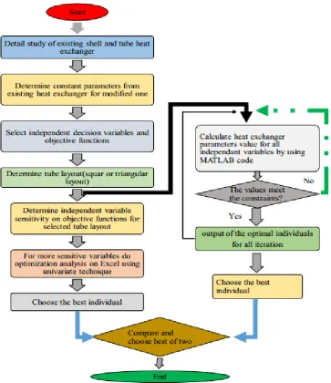
[image:2.595.114.478.218.639.2]Detail process of the design methodology considerations are shown in figurer 2.1.
Figure 2. 1 Flow chart for the research work
3. HEAT EXCHANGER MODEL AND DESIGN FORMULATION
To analyse the exchanger heat transfer problem, a set of assumptions are introduced so that the resulting theoretical models are simple enough for the analysis. The following assumptions are made for the exchanger heat transfer problem formulations:
The heat exchanger operates under steady-state conditions.
© 2019, IRJET | Impact Factor value: 7.34 | ISO 9001:2008 Certified Journal | Page 2630
There are no thermal energy sources or sinks in the exchanger walls or fluids.
The temperature of each fluid is uniform over every cross section in exchangers due to turbulence fluids are mixed enough.
Wall thermal resistance is distributed uniformly in the entire exchanger. Phase changes in the fluid streams flowing through the exchanger is negligible. Longitudinal heat conduction in the fluids and in the wall is negligible.
The fluid flow rate is uniformly distributed through the exchanger on each fluid side in each pass.
3.1
Design FormulationDepending on input parameters heat transfer analysis of an exchanger can be performed by using any of the -NTU or LMTD methods. Therefore in this heat exchanger heat transfer analysis –NTU method is used.
In the -NTU method, the heat transfer rate from the hot fluid to the cold fluid in the exchanger is expressed as
̇ ( )
, can be determined directly from the operating temperatures and heat capacity rates [3].
( )
( )
( )
( )
Where is the heat exchanger effectiveness, sometimes referred to as the thermal efficiency, is the minimum of ; =( ) is the fluid inlet temperature difference (ITD).
Heat Capacity Rate Ratio C* is simply a ratio of the smaller to larger heat capacity rate for the two fluid streams.
( ̇ )
( ̇ )
Number of Transfer Units NTU
The number of transfer units NTU is defined as a ratio of the overall thermal conductance to the smaller heat capacity rate [3]:
In general heat exchanger effectiveness is dependent on the number of transfer units NTU, the heat capacity rate ratio C*, and the flow arrangement for a direct-transfer type heat exchanger. Therefore for shell and tube, one shell pass (2, 4 . . . tube passes) arrangement heat exchanger effectiveness is represented as:
,
3.2. Overall Heat Transfer Coefficient
The equation basically sums up all the resistances encountered during the heat transfer and taking the reciprocal gives us the overall heat transfer coefficient [4].
(3.6)
(3.7)
Convection resistances and are calculated from the definition of convection resistance
© 2019, IRJET | Impact Factor value: 7.34 | ISO 9001:2008 Certified Journal | Page 2631
for in case of a tube of length and inner and outer diameters of Di and Do , from
(3.9)
Typical values of fouling resistance per surface area ( K / W) for the type fluid and the fouling layer resistance then obtained from [5]
(3.10)
From the above thermal resistance equations the value of U can be obtained.
̇ ̇
Wall resistance for circular tubes with a multiple-layer wall can be given by equation:
.∑
⁄
/
Where = wall thermal conductivity, = consecutive diameters between a layer and j = number of tube layers.
3.3. Fin Efficiency
Fins are generally used on the outside, but they may be used on the inside of the tubes in some applications. They are attached to the tubes by a tight mechanical fit, adhesive bonding, welding, or extrusion [6].
A logical definition of fin efficiency is therefore
̇ ̇
̇
(3.13)
( )
( ) ( ( ))
where is the surface area of the fin.
In contrast to the fin efficiency , which characterizes the performance of a single fin, the overall surface efficiency characterizes an array of fins and the base surface to which they are attached.
̇ ̇
̇
(3.17)
* ( ) +
© 2019, IRJET | Impact Factor value: 7.34 | ISO 9001:2008 Certified Journal | Page 2632
Where ̇ is the total heat rate from the surface area associated with both the fins and the exposed portion of the base (often termed the prime surface). If there are fins in the array, each of surface area A, and the area of the prime surface is designated as , the total surface area is
(3.23)
The maximum possible heat rate would result if the entire fin surface, as well as the exposed base, were maintained at Tb. The total rate of heat transfer by convection from the fins and the prime (unfinned) surface may be expressed as.
̇
Where the convection coefficient this assumed to be equivalent for the finned and prime surfaces [7].
Hence
3.4.Convective Heat Transfer Coefficient on Shell Side
The flow of gases over banks of finned tubes has been extensively studied and numerous correlations for this geometry are available in the open literature. Among these, the correlation of Briggs and Young has been widely used [8]:
⁄
⁄ ⁄ Where:
⁄
⁄
The Reynolds number is based on the tube outside diameter and the velocity on the cross flow area of the shell. = maximum air velocity in tube bank, =root diameter, = fin spacing, b = fin height, τ = fin thickness, = thermal conductivity of gas, = density of gas, µs = viscosity of gas, = gas-side heat-transfer coefficient
The fin spacing is related to the number, of fins per unit length by the following equation:
⁄
For an inline tube arrangement:
For the staggered tube arrangement:
*( ) +
̇
Where: face velocity the average air velocity approaching the first row of tubes, =pitch in the transverse, =pitch in the longitudinal tube row, =tube length, =the no flow dimension length.
3.5.Convective Heat Transfer Coefficient on Tube Side
© 2019, IRJET | Impact Factor value: 7.34 | ISO 9001:2008 Certified Journal | Page 2633
presented below are adequate to handle the vast majority of process heat-transfer applications [8].For heat-transfer coefficient, hi, the Seider–Tate and Hausen equations are used as follows.
For
⁄
⁄
For
* ⁄ + ⁄
( ⁄ ) (
⁄
)
For ,
( ) ⁄
( ⁄ )
Where
= Nusselt Number ≡ ⁄
= Reynolds Number ≡ ⁄
̇ ⁄
, ̇ = total mass flow rate of tube-side fluid, = number of tube-side passes, = number of tubes, ≡ Prandtl Number ≡ ⁄ = inside pipe diameter, = average fluid velocity, ⁄ = viscosity correction factor (dimensionless). But the value of ⁄ is approaches to 1, due to this mostly it is neglected and , , , = fluid properties evaluated at the average bulk fluid temperature.
3.6.Pressure Drop on Shell Side
The pressure drop for flow across a bank of tubes is given by the following equation:
Where: = Fanning friction factor, = number of tube rows, , ⁄ , , =the core length for flow normal to the tube bank and = minimum free-flow area.
For an inline tube arrangement:
For the staggered tube arrangement:
[( ) ]
=total heat transfer area both for fine and prime surface.
© 2019, IRJET | Impact Factor value: 7.34 | ISO 9001:2008 Certified Journal | Page 2634
For an inline tube arrangement:For the staggered tube arrangement:
⁄
( ) ⁄
, (
⁄ )
- ,
-
Where: ⁄ , ⁄ and
In addition to the tube bank, there are other sources of friction loss on the gas side. Although the friction loss due to each of those factors is usually small compared with the pressure loss in the tube bank, in aggregate the losses often amount to between 10% and 25% of the bundle pressure drop [3, 8].
3.7.Pressure Drop on Tube Side
The pressure drop due to fluid friction in the tubes with the length of the flow path set to the tube length times the number of tube passes. Thus,
Where: = pressure drop (Pa), = Darcy friction factor (dimensionless), L1 = tube length (m), = mass flux (kg /s · m2), s = fluid specific gravity (dimensionless), = viscosity correction factor (dimensionless) = ⁄ and for turbulent flow = ⁄ for laminar flow. But the value of is approaches to 1 due to this mostly it is neglected.
The minor losses on the tube side are estimated using the following equation:
( ) ⁄
For turbulent flow in commercial heat-exchanger tubes, the following equation can be used for Ret ≥ 3000:
For Ret 3000, laminar flow the friction factor is given by:
3.8. Cost Estimation
Cost is always an important consideration in designing any process equipment. In heat exchanger cost can be broken into two principal components – capital or investment cost and operating cost.
The capital cost for heat exchangers increases with increase in the heat transfer area whereas operating cost is primarily pumping cost. The pumps must provide work to overcome the pressure drop on the tube side and that on the shell side.
The operating cost Cop and the initial investment for the shell and the tube can be approximated as follows.
© 2019, IRJET | Impact Factor value: 7.34 | ISO 9001:2008 Certified Journal | Page 2635
Where, , are pressure factor, material factor, tube length factor and types of heat exchanger respectively.For carbon steel shell and steel tube materials
, a=1.55, b=0.05
Pressure factor =0.9876, for length 2.44 m.
, A is in m2
∑
Where Co is the annual cost, lifetime, and is the annual inflation rate.
The total operating cost is dependent on the pumping power to overcome the pressure drop from both shell and tube side flow [9].
( ̇ ̇ )
[image:8.595.68.527.391.758.2]Where the unit price of electrical energy, P is pumping power; H is the hours of operation per year and η is the pumping efficiency.
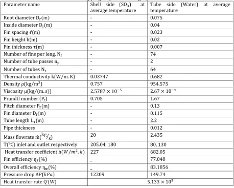
Table 3. 1 Existing (original) heat exchanger parameter values Parameter name Shell side ( ) at
average temperature Tube side (Water) at average temperature
- 0.075
Inside diameter - 0.04
Fin spacing ℓ(m) - 0.023
Fin height b(m) - 0.02
Fin thickness τ(m) - 0.007
Number of fins per leng. - 74
Number of tube passes - 2
Number of tubes - 64
Thermal conductivity k( ⁄ ) 0.682
Density ρ( ⁄ ) 954.575
Viscosity µ( ⁄ )
Prandtl number ( )
(m) - 0.13
Fin diameter - 0.115
Tube length (m) - 2.2
Pipe thickness - 0.012
Mass flowrate ̇( ⁄) 20 2.435
T inlet and outlet respectively , 180 80, 130
⁄ 227 682.05
Fin efficiency (%) _
Overall efficiency (%) _
Pressure drop ( )
© 2019, IRJET | Impact Factor value: 7.34 | ISO 9001:2008 Certified Journal | Page 2636
To select the best values to fulfil the objective functions, total cost evaluation has to be required. Functional years of original (existing) STHE ( annual discount rate (i) = 10 %, unit price of electrical energy in Ethiopia⁄ , Pump efficiency (The remaining days being nominal maintenance shutdown days).
From which total cost of original heat exchanger (CT) =1.8294 .
4.9. Selection of Decision Variables
Existing shell and tube heat exchanger has been studied above in detail. Standing from which the modified design STHE will be studied.
Impute data used in modified STHE is: Inlet and outlet temperature and mass flowrate of both fluids along with their physical properties, tube length, tube thickness, and length, width and height of the shell. Which is taken from the existing STHE because this heat exchanger is erected with in one frame with evaporator and erecting it alone and changing the shape is leading to another cost.
Here, the total cost and the heat transfer rate are the two objective functions. To fulfil the two neededobjective functions optimization problem should be required.
Optimization problem is exactly that, a problem for which the one want to select the best possible, optimal, solution from a set of alternatives.
The main objective of this optimization is to find out the minimum value for the total cost and maximum heat transfer rate of the heat exchanger simultaneously.
The existing shell and tube heat exchanger study was rating problem that stands from design parameters and some operating conditions with those unknown values operating parameters were calculated. But modified design will be opposite of this that is sizing problem.
Objective functions subjected to constraint taken from existing STHE heat transfer rate and total cost:
Q W and CT 1.8294
In modification, shell size is not considered because it is inter locked with evaporator and leads to additional cost.
So that modified STHE design decision variable parameters are reduced to:
Tube diameter ( )
Fin spacing (ℓ) Fin height (b) Fin thickness (τ)
Tube layout (triangular and square) Number of tubes
Number of rows
Number of passes
Pitch length
Number of fin
The variables listed above are both dependent and independent variables. The last five are dependent whereas the first five are independent variables. Since dependent variables can be expressed with independent values, it doesn’t need to change the values of dependent variables rather it can be varies whenever changing independent variables.
Due to these decision variables are decreased to five variables: fin space, fin height, tube diameter, Tube layout and fin thickness.
© 2019, IRJET | Impact Factor value: 7.34 | ISO 9001:2008 Certified Journal | Page 2637
Table 3.2 Comparison between square and triangular tube layoutsTube layout A U ̇
Square
(Existing) 64 2 94.54 227 0.39 513300 16 149.74 Triangular
(modified) 70 2 102.08 4207.6 221.86 103.37 0.54 715519.6 20 13857.22 146.22 U are expressed in ⁄ and ̇ ( ), and A
Here the table values were calculated from the same impute parameters that is fluids temperature, mass flow rate, tube length, tube diameter, tube thickness, number of fin, fin length, fin space, fin height and shell length, width and height. These results tells that number of tubes and rows increase due to compactness of the tube in triangular tube layout. Heat transfer area which is direct related to capital cost of STHE increases by 7.39 % whereas heat transfer coefficients in the tube and shell decreases because of decrease of Reynolds number. But overall heat transfer coefficient improved by 64.6 %. Heat transfer rate and performance of heat exchanger are raised by 39.4 and 37.17 % respectively with 13.5 % shell pressure drop penalty and 2.35 % tube pressure drop benefit.
Finally, conclusion can be drawn that triangular tube layout can be a good choice for modified shell and tube heat exchanger design if its parameters are adjusted in optimized way.
3.10. Sensitivity Analysis
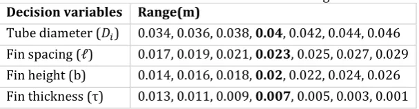
[image:10.595.147.451.408.487.2]Sensitivity analysis can be performed in order to observe the variation influences of design parameters over optimization objectives. Virational effects of four decision variables on the problem objectives of heat transfer rates and total cost of heat exchanger is shown below in Figure 3.1 to 3.4. Best solutions will be selected by influences of decision variables over problem objectives. The remaining variables stays constant during evaluations. Decision variables and their range of variation are listed in Table 3.3.
Table 3.3 Decision variables and their range Decision variables Range(m)
Tube diameter ( ) 0.034, 0.036, 0.038, 0.04, 0.042, 0.044, 0.046 Fin spacing (ℓ) 0.017, 0.019, 0.021, 0.023, 0.025, 0.027, 0.029 Fin height (b) 0.014, 0.016, 0.018, 0.02, 0.022, 0.024, 0.026 Fin thickness (τ) 0.013, 0.011, 0.009, 0.007, 0.005, 0.003, 0.001
Values written in the bold are taken from the existing STHE. To test the influence of decision variables over problem objectives back and forth of this values can be used.
Table 3.4 Diameter effects
Di A Ai U ∆Pfs ∆PTt
0.034 121.2632 27.00622 117.4943 797522.7 12475.31 327.1139
0.036 119.3312 27.3046 118.2336 794643.1 12583.11 292.1725
0.038 117.4376 27.54709 118.9084 791592.2 12684.63 262.4165
0.04 115.5827 27.73984 119.5268 788393.4 12780.23 236.9093
0.042 113.7665 27.88829 120.0955 785066.4 12870.24 214.9142
0.044 111.989 27.99726 120.6203 781627.7 12954.95 195.8455
[image:10.595.64.531.537.672.2]© 2019, IRJET | Impact Factor value: 7.34 | ISO 9001:2008 Certified Journal | Page 2638
Figure 3.1 Effects of diameter on objective functionsAs shown the fig. a-d above when internal diameter of the tube increases from 0.034 to 0.046 mm: overall heat transfer coefficient increase and blockage of gas in the shell is increase which leads pressure drop on the shell side are increasing in a small amount. Total area and heat exchanger effectiveness (heat transfer rate) decrease in a small amount. Here only pressure drop on the tube side is decreasing rapidly due to decrease of friction in the tube. The effects on heat transfer rate and heat exchanger effectiveness have the same profile since ̇ .
Table 3.5 Fin space effects
117
118
119
120
121
122
108
110
112
114
116
118
120
122
0.032
0.042
0.052
U (
W
/m
2.k)
A
(
m
2)
Tube diameter (m)
a
A
U
775000
780000
785000
790000
795000
800000
0.032
0.037
0.042
0.047
He
at
tra
nsfe
r
ra
te
(W
)
Tube diameter (m)
b
0.604
0.606
0.608
0.61
0.612
0.614
0.616
0.618
0.62
0.622
0.624
0.032
0.037
0.042
0.047
He
at
ex
cha
ng
er
ef
fe
cti
vne
ss
(ε
)
Tube diameter (m)
c
0
2000
4000
6000
8000
10000
12000
14000
0.032
0.037
0.042
0.047
P
re
ssure
dr
ops (Pa)
Tube diameter (m)
d
∆Pfs
∆PtT
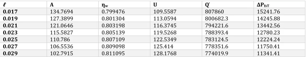
ℓ A ƞw U ∆PfsT
0.017 134.7694 0.799476 109.5587 807860 15241.76
0.019 127.3899 0.801304 113.0594 800682.3 14245.88
0.021 121.0646 0.803198 116.3745 794221.6 13442.56
0.023 115.5827 0.805139 119.5268 788393.4 12780.23
0.025 110.786 0.807109 122.5349 783124.5 12224.24
0.027 106.5536 0.809098 125.414 778351.6 11750.41
[image:11.595.31.566.600.700.2]© 2019, IRJET | Impact Factor value: 7.34 | ISO 9001:2008 Certified Journal | Page 2639
Figure 3.2 Effects of fin space on objective functionsFigure 3.2 shows that whenever the fin space increase from 0.017 to 0.029 mm:
Area of heat exchanger decrease due to fin area decrease.
Overall fin efficiency improved with a very small amount because of heat transfer area decrease but individual fin efficiency decrease.
Overall Heat transfer coefficient increase due to overall fin efficiency increase. Shell side pressure drop decrease due to less turbulence in the shell.
[image:12.595.36.564.617.748.2] But heat transfer rate decrease moderately compared to values on diameter.
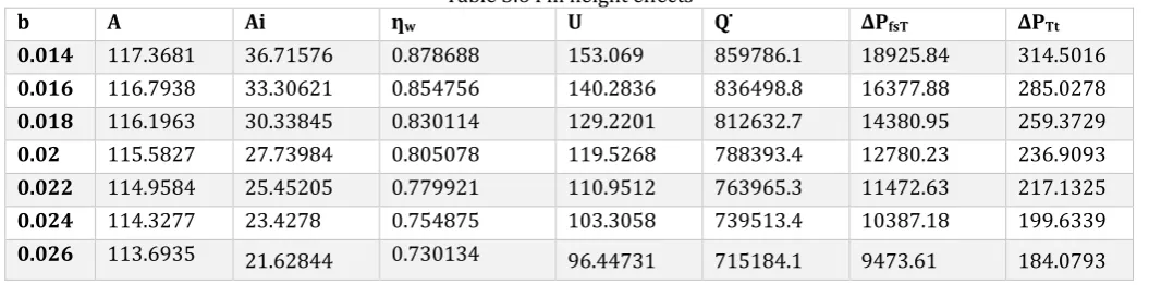
Table 3.6 Fin height effects
b A Ai ƞw U ∆PfsT ∆PTt
0.014 117.3681 36.71576 0.878688 153.069 859786.1 18925.84 314.5016
0.016 116.7938 33.30621 0.854756 140.2836 836498.8 16377.88 285.0278
0.018 116.1963 30.33845 0.830114 129.2201 812632.7 14380.95 259.3729
0.02 115.5827 27.73984 0.805078 119.5268 788393.4 12780.23 236.9093
0.022 114.9584 25.45205 0.779921 110.9512 763965.3 11472.63 217.1325
0.024 114.3277 23.4278 0.754875 103.3058 739513.4 10387.18 199.6339
0.026 113.6935 21.62844 0.730134 96.44731 715184.1 9473.61 184.0793
105
110
115
120
125
130
100
105
110
115
120
125
130
135
140
0.015
0.025
0.035
U (
W
/m
2.k
)
A
(
m
2)
Fin space (m)
A
U
770000
775000
780000
785000
790000
795000
800000
805000
810000
0.015
0.02
0.025
0.03
He
at
tra
nsfe
r
ra
te(
Ẇ
)
Fin space (m)
11000
11500
12000
12500
13000
13500
14000
14500
15000
15500
0.015
0.025
0.035
P
re
ssure
dr
op in t
he
shell (Pa)
Fin space (m)
0.798
0.8
0.802
0.804
0.806
0.808
0.81
0.812
0.015
0.02
0.025
0.03
Fin ef
icie
nc
y
(ƞw
)
© 2019, IRJET | Impact Factor value: 7.34 | ISO 9001:2008 Certified Journal | Page 2640
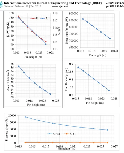
Figure 3.3 Effects of fin height on objective functionsTable 3.7 Effects of fin thickness
113
114
115
116
117
118
80
90
100
110
120
130
140
150
160
0.013
0.018
0.023
0.028
A
(
m
2)
U (
W
/m
2.K)
Fin height (m)
U
A
650000
700000
750000
800000
850000
900000
0.013
0.018
0.023
0.028
He
at
tra
nsfe
r
ra
te
(W
)
Fin height (m)
20
22
24
26
28
30
32
34
36
38
0.013
0.018
0.023
0.028
Ar
ea
of
tube(
m
2)
Fin height (m)
0.7
0.75
0.8
0.85
0.9
0.013
0.018
0.023
0.028
Fin ef
fic
ienc
y(ƞw
)
Fin height (m)
0
5000
10000
15000
20000
0.013
0.015
0.017
0.019
0.021
0.023
0.025
0.027
P
re
ssure
dr
ops (Pa)
Fin height (m)
∆PfsT
∆PtT
τ A ƞw U ∆PfsT
0.001 127.8344 0.563536 96.5455 753603.1 9508.287
0.003 123.1222 0.713878 109.7159 781634.5 10595.38
0.005 119.0832 0.774121 115.6901 787558.7 11687.29
© 2019, IRJET | Impact Factor value: 7.34 | ISO 9001:2008 Certified Journal | Page 2641
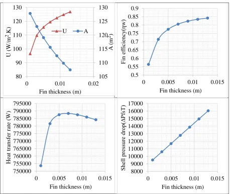
As shown values above from table and graph fin height has more variational effects. When fin height increase from 0.014 to 0.026 mm fin efficiency, heat transfer coefficient, heat transfer rate and pressure drop both on shell and tube side are increasing rapidly whereas total area change is small almost negligible. [image:14.595.69.528.172.558.2]Figure 3.4 Effects of fin thickness on objective functions
Table 3.7 and fig.3.4 shows that whenever fin thickness increases from 0.011 to 0.013:
Fin efficiency, heat transfer coefficient and shell side pressure drop also increases. But pressure drop increase more rapidly
Total surface area of STHE decrease.
Heat transfer rate first increases after a while it is decreasing but in a very small amount almost negligible.
In optimizing, the sensibility analysis needs to decide which adjustable variables of the problem are more important than others. Depending on sensitivities of variables over the objective functions, inside tube diameter and fin thickness have no significant effect on heat transfer rate. But fin height is more sensitive over the heat transfer rate and pressure drops which is related to operating cost. Fin space also more sensitive on heat transfer rate than fin thickness and diameter. Therefor from these result decision variables can be reduced to two decrease problem complexities that is:
Fin height and Fin space.
105
110
115
120
125
130
80
90
100
110
120
130
0
0.01
0.02
A
(
m
2)
U (
W
/m
2.K)
Fin thickness (m)
U
A
0.5
0.55
0.6
0.65
0.7
0.75
0.8
0.85
0.9
0
0.005
0.01
0.015
Fin ef
fic
ienc
y(ƞw
)
Fin thickness (m)
750000
755000
760000
765000
770000
775000
780000
785000
790000
795000
0
0.005
0.01
0.015
He
at
tra
nsfe
r
ra
te
(W
)
Fin thickness (m)
8000
9000
10000
11000
12000
13000
14000
15000
16000
17000
0
0.005
0.01
0.015
S
he
ll
pre
ssure
dr
op(∆
P
fsT)
Fin thickness (m)
0.009 112.5197 0.823193 122.4266 787529.6 13871.03
0.011 109.8171 0.834408 124.803 786003.8 14957.04
© 2019, IRJET | Impact Factor value: 7.34 | ISO 9001:2008 Certified Journal | Page 2642
By using these two decision variables design optimization of STHE can be performed.4. RESULTS AND DISCUSSION
4.1. Comparison of Univariate Results
From sensitivity analysis, all values of heat transfer rate and heat exchanger performances are greater than constraint values set above, which is due to change of tube layout. Therefore, for the next analysis calculated by the two decision variables (fin height and fin space) can be unconstrained univariate optimization type.
Table 4. 1 Selected decision variables and their range
Decision
variables Range(m)
Fin height (b) 0.011, 0.014, 0.017, 0.02, 0.023, 0.026, 0.029 Fin spacing (ℓ) 0.014, 0.017, 0.02, 0.023, 0.026, 0.029, 0.032
In Table 4.1, there are two variables,fin height (b) and fin spacing (ℓ) which have seven different values. By using these different values, 49 different alternative shell and tube heat exchanger can be found.
[image:15.595.43.542.361.749.2]These 49 different solutions are there. From which some required parameter values are single out and presented in Tables below.
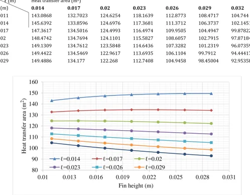
Table 4.2. Effects of fin height (b) and fin space (ℓ) over heat transfer area ℓ (m)
b (m)
Heat transfer area (m2)
0.014 0.017 0.02 0.023 0.026 0.029 0.032
0.011 143.0868 132.7023 124.6254 118.1639 112.8773 108.4717 104.744
0.014 145.6392 133.8596 124.6976 117.3681 111.3712 106.3737 102.1451
0.017 147.3617 134.5016 124.4993 116.4974 109.9505 104.4947 99.87822
0.02 148.4742 134.7694 124.1101 115.5827 108.6057 102.7915 97.87184
0.023 149.1309 134.7612 123.5848 114.6436 107.3282 101.2319 96.07359
0.026 149.4422 134.5469 122.9617 113.6935 106.1104 99.7912 94.44417
0.029 149.4886 134.177 122.268 112.7408 104.9458 98.45004 92.95358
Figure 4.1 Effects of fin height and space over heat transfer area
80
90
100
110
120
130
140
150
160
0.01
0.013
0.016
0.019
0.022
0.025
0.028
0.031
He
at
tra
nsfe
r
are
a
(m
2
)
Fin height (m)
ℓ=0.014
ℓ=0.017
ℓ=0.02
© 2019, IRJET | Impact Factor value: 7.34 | ISO 9001:2008 Certified Journal | Page 2643
As Figure 4.1 shows, for smaller constant fin space when fin height increase, fin area increase and base areas decrease with equivalent range as fin area due to number of tubes in the shell decrease. But the sum of the two that is total heat transfer area increase in a small amount. [image:16.595.48.542.180.555.2]For higher constant fin space when fin height increase, fin area increase in smaller range and base area decrease with a greater range than fin area. Therefore heat transfer area decrease for higher fin space.
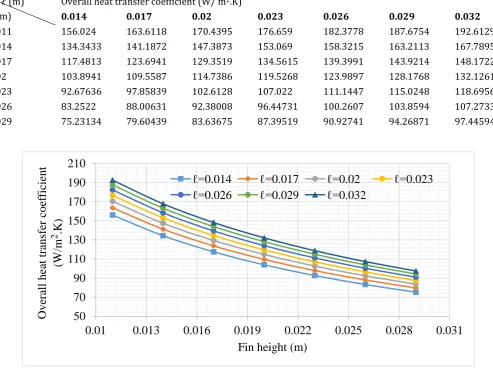
Table 4. 2 Effects of fin height (b) and fin space (ℓ) over overall heat transfer coefficient
ℓ (m) b (m)
Overall heat transfer coefficient (W/ m2.K)
0.014 0.017 0.02 0.023 0.026 0.029 0.032
0.011 156.024 163.6118 170.4395 176.659 182.3778 187.6754 192.6129
0.014 134.3433 141.1872 147.3873 153.069 158.3215 163.2113 167.7895
0.017 117.4813 123.6941 129.3519 134.5615 139.3991 143.9214 148.1722
0.02 103.8941 109.5587 114.7386 119.5268 123.9897 128.1768 132.1261
0.023 92.67636 97.85839 102.6128 107.022 111.1447 115.0248 118.6956
0.026 83.2522 88.00631 92.38008 96.44731 100.2607 103.8594 107.2733
0.029 75.23134 79.60439 83.63675 87.39519 90.92741 94.26871 97.44594
Figure 4. 2 Effects of fin height and space over heat transfer coefficient
Figure 4.2 tells that: At constant fin space, overall heat transfer coefficient decrease with increasing of fin height and at constant fin height heat transfer coefficient increase as fin space increase. But it increases with a small amount.
Table 4. 3 Effects of fin height (b) and fin space (ℓ) over fin efficiency
ℓ (m)
b (m) Overall fin efficiency (ƞ0.014 0.017 w) 0.02 0.023 0.026 0.029 0.032 0.011 0.905199 0.907663 0.910115 0.912507 0.914818 0.917037 0.919159
0.014 0.870785 0.873391 0.87606 0.878731 0.881365 0.883941 0.886447
0.017 0.834337 0.836963 0.839727 0.842555 0.845401 0.84823 0.851023
0.02 0.796912 0.799476 0.802244 0.805139 0.808102 0.811095 0.814088
0.023 0.759381 0.761831 0.764545 0.767438 0.77045 0.773534 0.776654
0.026 0.722428 0.724739 0.72736 0.730207 0.733216 0.736335 0.739525
0.029 0.686563 0.688725 0.691234 0.694006 0.696976 0.700089 0.703303
50
70
90
110
130
150
170
190
210
0.01
0.013
0.016
0.019
0.022
0.025
0.028
0.031
Ove
ra
ll
he
at t
ra
nsfe
r
coe
ffic
ient
(W
/m
2
.K)
Fin height (m)
© 2019, IRJET | Impact Factor value: 7.34 | ISO 9001:2008 Certified Journal | Page 2644
Figure 4. 3 Effects of fin height and fin space over fin efficiency [image:17.595.51.542.330.742.2]From figure 5.3: At constant fin space with increasing of fin height, fin efficiency is decreasing more rapidly.
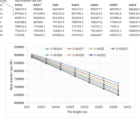
Table 4. 4 Effects of fin height (b) and fin space (ℓ) over heat transfer rate
ℓ (m) b (m)
Heat transfer rate (W)
0.014 0.017 0.02 0.023 0.026 0.029 0.032
0.011 906074.9 900850 896590.9 893115.7 890277.7 887959.7 886068.3
0.014 879461.9 871698.4 865215.6 859786.1 855224.5 851381.4 848136.5
0.017 850671.5 840509.6 831918.3 824624.7 818407.1 813086.5 808518.3
0.02 820188.6 807860 797367.9 788393.4 780679.6 774019.9 768247.5
0.023 788516.3 774300.1 762160.2 751732.7 742727.1 734911 728097.3
0.026 756147.4 740340.2 726821.5 715184.1 705105.9 696331.1 688654.6
0.029 723538 706435.1 691803.6 679195.5 668260.7 658722.5 650359.9
Figure 4. 4 Effects of fin height and fin space over heat transfer rate
0.6
0.65
0.7
0.75
0.8
0.85
0.9
0.95
0.01
0.013
0.016
0.019
0.022
0.025
0.028
0.031
Ove
ra
ll
fin e
ffic
ienc
y
(ƞw
)
Fin height (m)
ℓ=0.014
ℓ=0.017
ℓ=0.02
ℓ=0.023
ℓ=0.026
ℓ=0.029
ℓ=0.032
600000
650000
700000
750000
800000
850000
900000
950000
0.01
0.013
0.016
0.019
0.022
0.025
0.028
0.031
He
at
tra
nsfe
r
ra
te
(Ẇ
)
Fin height (m)
ℓ=0.014
ℓ=0.017
ℓ=0.02
ℓ=0.023
© 2019, IRJET | Impact Factor value: 7.34 | ISO 9001:2008 Certified Journal | Page 2645
Heat transfer rate: [image:18.595.49.545.168.585.2]At constant fin height with increasing of fin space, rate of heat transfer is decreasing in a very small amount especially for smaller fin height.
Table 4. 5 Effects of fin height (b) and space (ℓ) over pressure drop on the shell side
ℓ (m) b (m)
Pressure drop on the shell side (Pa)
0.014 0.017 0.02 0.023 0.026 0.029 0.032
0.011 31596.07 28352.97 26060.29 24349.31 23020.26 21955.61 21081.71
0.014 24990.63 22260.77 20346.14 18925.84 17827.79 16951.58 16234.69
0.017 20503.29 18161.02 16527.9 15321.74 14392.45 13652.94 13049.29
0.02 17284.76 15241.76 13823.87 12780.23 11978.26 11341.41 10822.44
0.023 14878.36 13071.72 11822.57 10905.66 10202.55 9645.12 9191.471
0.026 13019.34 11403.24 10289.36 9473.61 8849.147 8354.737 7952.808
0.029 11544.81 10085.14 9081.777 8348.401 7787.816 7344.483 6984.398
Figure 4. 5 Effects of fin height and fin space over pressure drop on the shell side Pressure drops:
Whenever the fin space increase at constant fin height, pressure drop decrease. But the rate of decreasing of pressure drop decrease.
At constant fin space decreasing of pressure drop rates are decrease with increasing fin height.
Now conclusion can be drown that at 32 mm fin space, pressure drops and heat transfer area are decreased with a small heat transfer rate penalty. But at constant 32 mm there are 7 alternative solution as yet. Which is
5000
10000
15000
20000
25000
30000
35000
0.01
0.013
0.016
0.019
0.022
0.025
0.028
0.031
P
re
ssure
dr
op on the she
ll
side (
P
a)
Fin height (m)
© 2019, IRJET | Impact Factor value: 7.34 | ISO 9001:2008 Certified Journal | Page 2646
Table 4. 6 Values at 32 mm fin space and variable fin heights.b A ƞw U Q ∆PfsT ∆PTt
0.011 104.744 0.919159 192.6129 886068.3 21081.71 367.6569
0.014 102.1451 0.886447 167.7895 848136.5 16234.69 314.5016
0.017 99.87822 0.851023 148.1722 808518.3 13049.29 271.7655
0.02 97.99125 0.814088 131.9791 768280.4 10592.62 215.4998
0.023 96.07359 0.776654 118.6956 728097.3 9191.471 208.1208
0.026 94.44417 0.739525 107.2733 688654.6 7952.808 184.0793
0.029 92.95358 0.703303 97.44594 650359.9 6984.398 163.8035
Figure 4. 6 Area, heat transfer coefficient, heat transfer rate, efficiency and pressure drops at a constant 32 mm fin space.
To select the best values to fulfill the objective functions, total cost evaluation has to be required. Functional years of original (existing) STHE ( annual discount rate (i) = 10 %, unit price of electrical energy ⁄ [Energy4sustainablefuture.blogspot.com], Pump efficiency
(The remaining days being nominal maintenance shutdown days).
0
50
100
150
200
250
90
92
94
96
98
100
102
104
106
0.01
0.015
0.02
0.025
0.03
U
(
W/
m
2.K
)
A
(
m
2)
Fin height (m)
A
U
600000
650000
700000
750000
800000
850000
900000
950000
0.01
0.015
0.02
0.025
0.03
He
at
tra
nsfe
r
ra
te
(W
)
Fin height (m)
0.6
0.65
0.7
0.75
0.8
0.85
0.9
0.95
0.01
0.015
0.02
0.025
0.03
Fin ef
fic
ienc
y
(ƞw
)
Fin height (m)
0
5000
10000
15000
20000
25000
0.01
0.015
0.02
0.025
0.03
B
oth pre
ssure
dr
op (Pa)
© 2019, IRJET | Impact Factor value: 7.34 | ISO 9001:2008 Certified Journal | Page 2647
Then by using cost estimation equations, 7 different alternative calculated values are listed in the table below.Table 4. 7 Investment cost, operating cost and total cost
b (m) ($)
0.011 72406.4275 3050221.19 3122627.61
0.014 71657.9338 2348930.64 2420588.58
0.017 71002.7095 1888049.46 1959052.17
0.02 61425.2315 1532500.12 1593900.35
0.023 69898.0155 1329880.1 1399778.12
0.026 69422.9297 1150663.3 1220086.23
[image:20.595.53.530.94.425.2]0.029 68987.2596 1010548.22 1079535.48
Figure 4. 7 Capital, operational and total cost of STHEX
Table 4.8 suggests that whenever fin height values varies from 11mm to 29 mm at constant 32 mm fin space there is no significant change on investment cost this means there is no significant change on heat transfer area. But not on operational cost. Figure 5.7 indicates that operating cost is the dominant cost factor in a shell and tube heat exchanger. Even if it incorporates pumping cost for hot and cold fluids, the dominant factor for this cost is pumping cost of hot fluid in the shell. As a result to minimize total cost it is better to focus on pressure drop in the shell which is responsible for operational cost.
4.2 Dual Objective Optimization Using Univariate Method
As mentioned, dual objective optimization yields Pareto solutions that constructs the Pareto curve. It can also be said that a favorable trade-off between the results of contradictive objectives is called Pareto optimum solution. Figure 5.8 and 5.9
shows the Pareto frontier constructed by the dual objective optimization of abovementioned problem objectives.
Table 4. 8 Pareto optimal solution
CT ($) ̇ (W)
3122627.61 886068.3
2420588.58 848136.5
1959052.17 808518.3
1593900.35 768280.4
1399778.12 728097.3
1220086.23 688654.6
1079535.48 650359.9
0
500000
1000000
1500000
2000000
2500000
3000000
3500000
0.011
0.014
0.017
0.02
0.023
0.026
0.029
C
osts
($)
Fin height (m)
© 2019, IRJET | Impact Factor value: 7.34 | ISO 9001:2008 Certified Journal | Page 2648
Figure 4. 8 Pareto curve of objective functionFigure 4. 9 Heat transfer rat and total cost at different fin height
Univariate optimization technique was implemented using Excel to get optimal solutions and for these optimal solutions Pareto analysis is required to decide important adjustable variables. As shown Figure 5.8 on the Pareto curve which indicates the conflict between total cost and heat transfer coefficient that is at point A both cost and heat transfer rate are minimum whereas at point G both objective functions are maximum.
550000
1050000
1550000
2050000
2550000
3050000
3550000
600000
650000
700000
750000
800000
850000
900000
950000
T
otal c
ost ($)
Heat transfer rate (W)
A
B
C
D
E
F
G
0
100000
200000
300000
400000
500000
600000
700000
800000
900000
1000000
100000
600000
1100000
1600000
2100000
2600000
3100000
3600000
0.01
0.013
0.016
0.019
0.022
0.025
0.028
0.031
He
at
tra
nsfe
r
ra
te
(W
)
T
otal c
ost ($)
[image:21.595.70.528.395.670.2]© 2019, IRJET | Impact Factor value: 7.34 | ISO 9001:2008 Certified Journal | Page 2649
Figure 4.9 indicate that whenever increasing fin height from 11 mm to 29 mm heat transfer rate decrease almost in equal ranges, while total cost drops rapidly for the first some values. But the range of decreasing values become decrease with fin height.Finally, from Pareto optimal point solutions one point can be selected for constraint of ̇ ≥ 5.133 105 W and CT ≤ 1.8294 106 $. Due to this, it is acceptable to choose design point D at ̇=7.6828 105 W and CT=1.5939 106 $ as modified design of shell and tube heat exchanger of for univariate optimization method.
[image:22.595.142.450.192.414.2]4.3 Dual Objective Optimization Using ACO
Figure 5. 10 Total cost Vs heat transfer rate Pareto fronts of STHEs without constraints.
[image:22.595.146.447.485.717.2]When constraint parameters are excluded (non-constraint optimization) as shown Figure 5.10, 2,401 alternative number of STHEs which represented with its’ total cost and heat transfer rate can be found by using MATLAB code.
© 2019, IRJET | Impact Factor value: 7.34 | ISO 9001:2008 Certified Journal | Page 2650
Figure 4. 12 Total cost Vs heat transfer rate Pareto front of STHEs with constraint of ̇ ≥ 5.133 105 W and CT ≤1.8294 106 $.
As Figure 4.10, the stares in Figure 4.12 also shows different alternative STHEs. But it has constraint parameters of ̇ ≥ 5.133 105 W and CT ≤ 1.8294 106 $ which is taken from existing STHE. Due to this number of alternative, STHEs are decreased from 2,401 to 1,280. Of which one optimum point with the smallest total cost to heat transfer rate ratio (CT/ ̇ = 1.4795) is selected. At this point total cost and heat transfer rate are 1.1463 and 7.74810 W respectively.
Figure 4. 13 Total cost Vs heat transfer rate Pareto front of STHEs with constraint of ̇ ≥ 7.6828 105 W and CT ≤ 1.5939 106 $.
[image:23.595.123.461.443.671.2]© 2019, IRJET | Impact Factor value: 7.34 | ISO 9001:2008 Certified Journal | Page 2651
Design optimization of heat exchanger by using Univariate and ACO have different optimal values. Existing parameter values and modified STHE optimal point values both in Univariate and ACO are listed below in Table 4.9.Table 4. 9 Both existing and modified exchanger parameter values
Heat exchanger parameters
Existing STHEX values
Modified STHE values (Univariate method )
Modified STHEX values (ACO method)
(m) 0.115 0.096 0.09
Root diameter (m) 0.075 0.056 0.05
Tube diameter (m) 0.04 0.04 0.034
Fin space ℓ(m) 0.023 0.032 0.029
Fin height b(m) 0.02 0.02 0.02
Fin thickness τ(m) 0.007 0.007 0.003
(m) 74 55 31
Number of tube (m) 64 102 114
Number of pass (m) 2 3 3
Number of tube per pass 32 34 38
Number of row (m) 16 23 21
Heat transfer area A( ) 94.54 97.991247 110.7173
Heat tran. coef. in tube ( ⁄ ) 696.6 4216.76577 5168.7
Heat tran. coef. in shell ( ⁄ ) 227 240.7993642 246.8468
Overall heat trans.coef U( ⁄ ) 63.5 131.9791486 119.3063
Heat exchanger performance ε 0.3811 0.598474276 0.6036
Heat transfer rate ̇(W) 5.27 7.6828 7.7481
Pressure drop in shell ∆ ( ) 10.5926232 7.5361
Pressure drop in tube ∆ (Pa) 156.861 215.4997537 448.3515
Number of tubes per rows
(for odd and even respectively) 4, 4 5, 4 6, 5
Investment cost 6.3102 6.1425 5.6051
Operating cost 1.7663 1.5325 1.0903
Total cost CT($) 1.8294 1.5939 1.1463
The existing design and the modified STHE obtained using Univariate optimization approach and ACO method results are summarized in Table 4.9. The table demonstrates that the Univariate design approach and the ACO design approach can reduce the total cost compared to the original design approach. Quantitatively, a remarkable reduction in the total cost was achieved using the Univariate approach (by 12.87 %) and the Ant Colony Optimization approach (by 37.34 %) as compared to the original design, whereas heat transfer rate increased by 45.78 % and 47.02 % by using Univariate and ACO method respectively as compared to the original design. Therefore, design optimization of modified STHE by using ACO approach can be the best choice. The results found from univariate and ACO were selected from 49 and 2,401 alternative STHEs respectively. To get the same result in univariate technique as ACO values, Univariate technique needs 2,401 trials on Excel spreadsheet. But it is tedious and takes time and also leads to input data as well as output analysis error. That is why sensitivity analysis is used to avoid this challenge.
Result Validation
The present results in both of the optimization methods are able to provide equivalent STHE design to the related reference [9].
© 2019, IRJET | Impact Factor value: 7.34 | ISO 9001:2008 Certified Journal | Page 2652
Whereas the present work calculated for a fined STHE using a multi-objective optimization ACO and Univariate methods for the decision variables (tube arrangement, tube diameter, fin height, fin thickness and fin space) involved in optimization of the objective functions (maximum heat transfer rate and minimum total cost). The equipment life was taken ny =20 years; and the working hours H = 8040 h/year.As shown figure 4.14, distribution of Pareto-optimal point solutions in 4.14a forms a curve line because in genetic algorisms each iteration results are updated in the next iterations.
In ACO, Pareto-optimal point solutions are randomly distributed, because of all iteration outputs are displayed. But as shown figure 4.14 all graphs have similar trend. Finally, by considering those conditions which make difference, these multi objective optimization methods for STHE design can be validated against the reference cases in the literature [9].
a). The distribution of Pareto-optimal point solutions using NSGA-II [9]
© 2019, IRJET | Impact Factor value: 7.34 | ISO 9001:2008 Certified Journal | Page 2653
c). The distribution of Pareto-optimal point solutions using Univariate methodFigure 4. 14 Validation of present results against the reference cases in the literature
5. CONCLUSIONS
In this paper detail study of existing shell and tube heat exchanger and a modified multi-objective optimization design approach is proposed for the shell and tube heat exchanger on Microsoft Excel using univariate and ACO optimization technique with the objective functions of maximizing heat transfer rate and minimizing total cost using MATLAB. Five independent decision variables are considered, including tube arrangement, tube diameter, fin height, fin thickness and fin space. Of which, tube diameter and fin thickness have less significant change over heat transfer rate and multi objective optimization for the modification of a shell-and-tube heat exchanger allowed finding Pareto fronts with optimal decision variables both in Univariate(in Excel) and ACO(in MATLAB) techniques. From which it can be chosen one solution from all Pareto optimal solutions based on heat transfer rate as well as the cost of the design for both techniques. In Univariate and ACO methods, heat transfer rate (7.6828 ) and total cost (1.5939 and 1.1463 ) respectively have been selected.
Finally result shows that:
The tube arrangement and fin height have more significant effects on heat transfer rate and cost of STHE.
Operating cost is the dominant cost factor in a shell and tube heat exchanger.
Within operating cost, pressure drop in the shell is a dominant factor.
Heat transfer rate in both techniques have almost the same values, but it has significant difference in total cost.
ACO approach is more cost-effective than Univariate (traditional) optimization technique.
Optimal point selected from Pareto optimal solutions of modified STHE in ACO approach was improves heat transfer rate by 47.02 % and total cost reduction by 37.34 % when compared with existing shell and tube heat exchanger.
6. REFERENCES
[1]. Shravan H. Gawande, Sunil D. Wankhede, Rahul N. Yerrawar, Vaishali J. Sonawane and Umesh B. Ubarhande, Design and Development of Shell and Tube Heat Exchanger for Beverage, Modern Mechanical Engineering, 2012, 2, 121-125.
[2]. Shah, R. K, Classification of Heat Exchangers, 1981.
550000
1050000
1550000
2050000
2550000
3050000
3550000
600000
650000
700000
750000
800000
850000
900000
950000
T
otal c
ost ($)
Heat transfer rate (W)
A
B
C
D
E
F
© 2019, IRJET | Impact Factor value: 7.34 | ISO 9001:2008 Certified Journal | Page 2654
[3]. Ramesh K. Shah, Fundamental of Heat Exchanger Design, Rochester Institute of Technology, Rochester, New York,2003.
[4]. Usman Ur Rehman, Heat Transfer Optimization of Shell-and-Tube Heat Exchanger through CFD Studies, Chalmers University of Technology, G Oteborg, Sweden 2011.
[5]. Piyush Gupta, Avdhesh Kr. Sharma and Raj Kumar, Thermal Design of Shell and Tube Heat Exchanger Using Elliptical Tube, International Journal of Engineering and Manufacturing Science. ISSN 2249-3115 Vol. 7, 2017. [6]. R. K. Shah, Heat Exchangers, in Encyclopedia of Energy Technology and the Environment, edited by A. Bisio and
S. G. Boots, pp. 1651-1670, John Wiley & Sons, New York, 1994.
[7]. Frank P. Incropera, Theodore L. Bergman, Adrienne S. Lavine and David P. Dewitt Fundamentals of Heat and Mass Transfer, Seventh Edition, 2011.
[8]. Robert W. Serth, Process Heat Transfer Principles and Applications, Texas A&M University-Kingsville, Kingsville, Texas, USA, First edition 2007.
[9]. Heidar Sadeghzadeh, Mehdi Aliehyaei and Marc A. Rosen, Optimization of a Finned Shell and Tube Heat Exchanger Using a Multi-Objective Optimization Genetic Algorithm, ISSN 2071-1050, 25 August 2015.
NOMENCLATURES
List of Symbols and Abbreviations Symbols
̇ heat transfer rate [W] number of fins [-]
̇ ̇ mass flow rates [kg/s] h convective heat transfer rate [W/ K]
specific heats [J/kg.K] [-]
outlet temperatures [ ] Reynolds- number [-]
inlet temperatures [ ] maximum air velocity in tube bank overall heat transfer coefficient [W/ K] root diameter [m]
log mean temperature difference [-] ℓ fin spacing [m] F the correction factor of heat transfer rate [-] b fin height [m]
fouling resistance per surface area [ K / W] τ fin thickness [m]
total resistance [K/W] k thermal conductivity [W/m.K]
resistance tube wall [K/W] µ dynamic viscosity [kg/s.m]
̇ fin heat transfer rate [W] Gas-side heat-transfer coefficient
[W/ K]
Ε heat exchanger effectiveness [-] pitch distance [m]
area at the base of the fin [ ] root diameter [m]
temrature difference between the base and free
stream [ ] face velocity the average air velocity approaching the first row of tubes [ ] free stream temperature [ ] prandtl number, surface roughness term
[-]
the surface area of the fin [ ] density [kg/ ]
fin efficiency [%] pressure drop for flow across a bank of
tubes [Pa]
overall surface efficiency [%] pressure drop for flow in the tubes [Pa]
̇ total heat rate from the surface area A, associated with both the fins and the exposed portion of the base [W]
f fanning friction factor [-]
G mass flux [kg/ ] number of tube rows [-]
fin outside diameter [m] the core length for flow normal to the tube bank [m]
© 2019, IRJET | Impact Factor value: 7.34 | ISO 9001:2008 Certified Journal | Page 2655
pitch in the longitudinal tube row [m] s fluid specific gravity [-]tube length [m] viscosity correction factor [-]
the no flow dimension length [m]
Subscript
hot fluid free stream
cold fluid Root
Inlet Maximum
Outlet min. Minimum
Fin t in the tube
Base s in the shell
ABBREVIATION
AMASSAS.Co Awash Melkassa Aluminum Sulfates and Sulfuric Acid Share Company
STHE Shell and tube heat exchanger
NTU Number of transfer unit
ACO Ant colony optimization
BIOGRAPHIES
Melkamu Embiale was born in July in 1993. He received the B.Sc. degree in Mechanical Engineering (Thermal) and the M.Sc. degree in Thermal Engineering from Adama Science and Technology University, Ethiopia, in 2016 and 2019, respectively.
Dr. Addisu Bekele (Corresponding Author) was born in Ethiopia on 10th May 1985. He Completed
Dr. Mohanram Parthiban, born in Sendamangalam, Namakkal (DT), Tamilnadu, India on 19th June 1978, Completed Bachelor of Engineering (Mechanical Engineering) in the year of 2000, completed Master of Engineering (Thermal Engineering) in the year of 2004 and ompleted PhD (Thermal Engineering) in the year of 2015. He has published four articles in international journal, an article in international conference and two articles in national conferences. His research area is heat transfer, solar energy and thermal energy storage systems.
Dr. Chandraprabu Venkatachalam was born in Tiruchengode, Namakkal (DT), Tamilnadu, India on 25th January 1977, Completed Bachelor of Engineering Mechanical Engineering) in the year of 1999, completed Master of Engineering (Thermal Engineering) in the year of 2005 and completed PhD (Thermal Engineering) in the year of 2014. He has published nine articles in international journal, three articles in international conference and seven articles in national conferences. His research area is heat transfer enhancement in air conditioner using nano fluids and solar energy.