An Autoregressive Integrated Moving Average Models For Process Output And Forecasting

(1)

RESEARCH ARTICLE

AN AUTOREGRESSIVE INTEGRATED MOVING AVERAGE MODELS FOR PROCESS

OUTPUT AND FORECASTING

ADARABIOYO, M. I

Statistics Department, Achievers University, PMB 1030, Owo, Ondo State

ARTICLE INFO ABSTRACT

In the first stage of analysis, some descriptive measures were used to examine the main properties of the series. Twelve-month centred moving average and differencing of order twelve advocated by Box and Jenkins (1970) were used to reduce the seasonal effect and to make the series stationary respectively. The autocorrelation of the differenced series of the productions were calculated including the partial autocorrelation with their respective correlogram which gives an insight into the probability model that generated the series.The second stage involves fitting of model and diagnostic checking to test for the adequacy of the fitted model. The diagnostic checking revealed that autoregressive model of order two was fitted into the series.

INTRODUCTION

Time Series analysis is an effective tool that can be used to achieve production goals in any Organization. It can be used to make short and long time decisions even more importantly for long time planning and forecasting the future tendency.

Most economic data are measured over time. A time series, therefore, ‘‘is a collection of observations made sequentially over time’’. In the economic sector, we observe share prices on successive days, export totals in successive months, average incomes, and company profits in successive years, and so on. In Agriculture, we observed annual rain-fall, production and profit and so on. In engineering we observed sound, electric signals and voltage. In Geophysics, we observe turbulence such as ocean waves and earth noise in an area. We can also monitor a process according to a certain target value. Time series such as the measurement of sound, electric signals and voltage which can be measured and recorded continually in time is said to be a continuous time series. When observations are taken only at a specific time usually equally spaced even when the measured variable is continuous, series of this type is said to be discrete. In addition, time series can be stochastic or deterministic. A stochastic process can be described as a random element in their structure. A stochastic process can be described as a statistical phenomenon that evolves in time according to probabilistic laws. That is future values can be predicted from past observations. Deterministic series occur only if the future values can be predicted by some mathematical functions.

*Corresponding author: marydo2004@yahoo.com

If the future values can be described only in terms of a probability distributions, the series is said to be non-deterministic or simply a statistical time series.

In Engineering the word ‘’spectral’’ or ‘’frequency domain’’ is frequent. While in Mathematical statistics, correlation’’ or ‘’time domain’’ is also frequent. The spectral properties of stationary models is the analysis of time series based on the assumption that it is made up of

sine and cosine waves with different frequencies (Priestly, 1981). A device which uses this idea, first

introduced by Schuster (1998) is the periodogram. The periodogram was originally used to detect and estimate the amplitude of a sine component of known frequency, buried in noise.

Several books have been written on time series analysis. Their writings were based on theoretical aspects of time series analysis and are mainly concerned with mathematical theory. Another author who made an immeasurable contribution to time series analysis literature is Box and Jenkins (1970). The book describes the approach of time series analysis, forecasting and control. It is based on a particular class of linear stochastic models.

Several Researches had been carried out involving the use of autoregressive integrated moving average. Among these is in Epidemiology, Allard. (1998) worked on the uses of time series analysis in infectious surveillance and Ernest (2005) who worked on Autoregressive Integrated Moving Average Model to predict and monitor the number of beds occupied during a SARS outbreak in Singapore. The essence of this research is to see its practicability in Manufacturing Industry such as the Global Soap and Detergent Ilorin, Kwara State, Nigeria.

ISSN: 0975-833X

International Journal of Current Research Vol.7, pp.049-054, August, 2010

INTERNATIONAL JOURNAL

OF CURRENT RESEARCH

Series, Stationary, Autocorrelation, Autoregressive, Diagnostic, Forecasting

Article History:

Received 23rd_{April, 2010} Received in revised form 27th June, 2010 Accepted 18th_{July, 2010}

(2)

MATERIALS AND MOTHODOLOGY

The data used in this research work was collected from the statistics unit of the Global Soap and Detergent (Nig) Limited, Ilorin Factory, Ilorin Kwara State. The data was available on monthly basis and it covered a period of Ten years. There are basically two approaches to the analysis of discrete time series. The approach to be used depends on the object of the analysis. These two methods are the traditional and the stochastic methods. The traditional method concerned the decomposition of time series into its various components. Observations recorded over time are assumed to be influenced by some factors such as seasonal fluctuations, cyclic components, irregular, trends and so on. One or more of these components may be absent but the irregular component is always present. Assumptions about the combination nature of the factors enable us to fit suitable model to a series. Two practical methods; additive and multiplicative models are often used.

Autoregressive Integrated Moving Average Models

The general autoregressive integrated moving average process of order (p,d,q) denoted by

ARIMA(pdq):

_

_

_

_

_

q t q t t p t p t t

t W W W

W 1  1 1...   1... 

… (6) where



 dyt t

W

is the differenced series and ,

... , , .. ,

2 1 2

1







q

p

are as defined above

Model Selection

Three stages iterative procedure based on specification, estimation and diagnostic checking are used to obtain an appropriate model.

Specification

This is the use of data and any information on how the series was generated, to suggest a subclass of parsimonious models worthy to be entertained. In achieving this time plot autocorrelation function, correlogram, test for randomness or stationary and the main partial autocorrelation functions are used to obtain the main properties of the series.

Autocorrelation Function

The sample autocorrelation coefficients measure the correlation between adjacent observations at different distances (lag apart). These coefficients often provide insight into the probability model that generated the series the autocorrelation coefficients



k at lag k is given by:

rk=

C

Y

k K

N

t K N

t t t k

t N

Y Y

K N

0

1

2 1

)

(

1

) )( ( 1

  











 

  …………..(7)

Ck=



 

  



K N

t

k t

t Y Y

K

N 1

Y

) )(

(

1 _{………….(8)}

= autocorrelation coefficient at lag K

Time Plot Showing Monthly Production values

0 100000 200000 300000 400000 500000 600000 700000

0 50 100 150

Time

P

r

u

d

u

ct

io

n

Production values

Correlogram of Autocorrelation of the Monthly Production

-0.2 -0.1 0 0.1 0.2 0.3 0.4 0.5

0 10 20 30 40

Correlogram

Trends of Monthly Production

0 50000 100000 150000 200000 250000 300000 350000 400000 450000

1 5 9 13 17 21 25 29 33 37 41 45 49 53 57 61 65 69 73 77 81 85 89 93 97

Time

P

r

o

du

c

t

ion

Correlogram of Autocorrelation

of Differenced Series

-0.5

0

0.5

1

4

7 10 13

Lag

A

u

to

c

o

rr

el

at

io

n

co

e

ff

ic

ien

t

(3)

-0.4 -0.2 0 0.2 0.4 0.6 0.8 1

1 6 11 16 21 26

P a rt ia l a n d A u to c o rr e la ti o n c o rf fi c ie n ts Lag Correlograms of Autocorrelation and Partial

Autocorrelation of monthly production

Autocoefficients

partial autocoeeficients

And

C0=





 

K N

t

Y

t

Y

N 1

2

)

(

1 _{…..………..(9)}

= sample variance, which is equivalent to auto-covariance at lag zero.

Partial autocorrelation function

The partial autocorrelation function enables ones to know which order of autoregressive process to fit an observed time series. A recursive formula for calculating the partial autocorrelation is given by:

If K=1                  



    K N

t k k

K N

t k k

k kk

r

j N j N 1 1 , 1 1 1 1 , 1 1



………(10)

If K = 2 ,…, L

Correlogram

A useful aid in interpreting a set of autocorrelation coefficient,



k, is a graph called the correlogram in

which



kis plotted against the lag k. for a non-stationary

time series, the values of



kwill not come down to zero

except for very large values of lag, whereas for a stationary time series, the values of



kwill come down to

zero and the model is assumes that the process remains at equilibrium about a constant mean level.

Test for randomness and stationary

If any time series data are completely random for large N,



_k= 0, for all non-zero values of K, Box and Jenkins (1970) showed that in searching for significance of



k,

the values



k which lie outside the range

_N

2 

are certainly significantly different from zero and need further investigation.

Parameters estimation

The estimation of autoregressive model is described below:

For a process



kassumed to have a non-zero mean. A

suitable model for AR(p) is





t t p t p t

t

W

 _ _₂... _ 

2 1

1 ………..(11)

Where

Wt = Yt – U and



p

..

,

2

1 a are constant

Given N observations r1, r2,..,rN, the problems is to

estimate the unknown parameters



p

..

,

2

1 and



.

The equation can be written as





t t p t p t

t

W

 _  _₂... _ 

2 1 1

…………(12) There is superficial similarity between equation (12) and the classical multiple regression models. Wt is expressed as a linear function of

W

t1 t2

..

tp With



pacting as the regression

coefficients and



_t is the ‘’residual’’.

Since the values r1, r2, …, rN, are all observed there is

nothing preventing the application of least squares procedure used in regression analysis. The estimates



,

..

_p

2

1 are obtained by minimizing;



 



N p t t

S

1 2

)

(



_

) ... ( 1 1 1



       N p t p t p t

t

W



2 …(13)

The summation takes values from t= p+1 because the terms



2



2

1

,...,

p can not be computed in terms of the

observed.

Other methods are the use of exact likelihood function and the use of Yule-Walker’s equation provides estimate that are approximately to the least squares estimates and to the maximum likelihood estimate. The Yule-Walker’s estimates are ) ,..., ( , 2 1 1



p r

R



  ……….(14)

                1 ... 1 2 1 2 1 1 .... 1

r

p p p p _and

                

r

p r . . 2 1



   



N p t t N p t t

e

a

S

1 2 1 2

)

(



……….(15)

is estimated by either forward or backward equation. The forward equation is given by

at=

W

p t p t

t

t



1 1



2 2...





……(16) And the backward equation is given by

et

_W

p t p t

t

t     





...



2 2 1 1 …………..(17) Where (at)’s and the (et)’s the error terms.

Hence the initial estimate of the autoregressive process of order one is given by





1

(4)

where the initial estimate for and of the second order autoregressive process obtained from









1

2

1 2 1 1

)

(

and









1

₁2

2

1 2

2 .

The admissible region of stationary is given as

1 1 1 1

1 2

1

 

 

  



For autoregressive process of order one,





1



= 0.419 and second order autoregressive process we have

Table1. Autocorrelation coefficients ofmonthly production

Lag Autocorrelatio

n coefficients

Lag Autocorrelation

coefficients

1 0.419 11 0.205 21 0.11

2 0.24 12 0.211 22 0.127

3 0.24 13 0.258 23 0.114

4 0.251 14 0.227 24 0.061

5 0.237 15 0.092 25 0.092

6 0.221 16 0.084 26 0.134

7 0.267 17 0.199 27 0.053

8 0.268 18 0.159 28 0.046

9 0.301 19 0.184 29 -0.106

10 0.256 20 0.132 30 -0.046

Table 2. Autocorrelation coefficients of differenced series

coefficients(rk)

La g

Autocorrelation coefficients

La g

Autocorrelation coefficients(rk)

1 0.191 11 -0.150 21 -0.048

2 0.175 12 -0.250 22 0.031

3 0.149 13 -0.030 23 0.022

4 0.055 14 -0.102 24 0.082

5 0.049 15 -0.097 25 0.005

6 0.033 16 0.21 26 -0.063

7 0.068 17 0.77 27 -0.027

8 0.119 18 -0.026 28 -0.062

9 0.126 19 0.073 29 -0.076

10 0.027 20 -0.260 30 0.021

Table 3. First oeder autoregressive process

ITERATION PARAMETER(



) SSE(



) MSE(



)

0 0.419 1.07466E+12 9.1073E+9

1 0.519 1.08754E+12 9.4282E+9

2 0.619 1.09233E+12 9.6354E+9

3 0.719 1.19136E+12 9.9237E+9

4 0.819 1.28231E+12 9.9991E+9

Table 4. Second oeder autoregressive process

ITERATION PARAMETERS(



k)



₁



2

SSE(



) MSE(



)

0 0.325 0.148 1.04123E+12 8.7498E+9

1 0.325 0.248 1.04298E+12 9.1392E+9

- - - - -

(5)









1

2

1 2 1 1

)

( _=0.325and







 

1

12 2

1 2

2

=0.148. …..(18)

The parameters satisfied the admissible region of stationary.

Diagnostic Checking

Box and Jenkins (1970), described a check called portmanteau lack-of-fit test is given by

)

(

1 2

a

r

t

k

t k

N

Q

_



; ……….(19)

Where, N is the number of the observations and



















 





K N

t K N

t

k t k k

a

r

t

N

1 2 1

1

is the autocorrelation

coefficient of the residuals obtained from the fitted model

Q

is approximately distributed Chi-square with N-p-q degrees of freedom. Where (p, q) and N-p-q are number of orders in the AR and MA terms respectively.

Mean Square Error Method

After diagnostic check, the best model can be selected using the Mean Square Error Method (MSE). The MSE is computed thus:

MSE =

p

N

S



)

(



where

S

(



)

is the sum of squares error and N-p is the error degrees of freedom N is the number of observations and p is the number of estimated parameters.

RESULTS AND DISCUSSION

The time plot is characterised by recurring up and downward movement which indicates the presence of secular trend, irregular and seasonal variations. The variations is an indication of the presence of permanent force which operating uniformly (Figure 1). Using the SPSS, thirty (30) autocorrelation coefficients were obtained (Table1) which agrees with the general rule of N/4 autocorrelation values from N observations (N = 120). A critical look at the correlogram (Figure 2) reveals that the autocorrelation coefficients are significance at lags 1, 2, …, 14 and 19. These values were outside the limit of



2 /

N





0 .

183

. Thus indicating the presence of seasonal and trend effect with some irregular variations that cannot be identified. In order to remove the seasonal effect, a 12-order moving average was used. The trend of the 12-month moving average did not follow a particular pattern which may be due to the presence of irregular variation which has not been fully eliminated (Figure 3). Consequent upon the above, a difference of order twelve that is

_Y

_t_₁₂



_Y

_t

,

_Y

_t_₁₃



_Y

_t_₁

,...

, was carried out for the purpose of obtaining a stationary model. The autocorrelation of the differenced series yields the autocorrelation coefficients in Table 2 with the

corresponding correlogram in figure 4. The values of rk

remain significance after the twelve order differencing. However, according to Chatfield (1975), one is expected to find at least one value of the autocorrelation of the differenced to be significant even when the series is stationary. Based on this assumption, the values of rk that

lies outside the limits rk



2 /

N





0 .

183

are due to

irregular variations and that the series is stationary. In order to specify an appropriate production model, the partial autocorrelation coefficients of the production values were computed with the aid of SPSS and the values compared with the autocorrelation coefficients with their corresponding correlograms (Table3) and (Figure 5). Greater values of the partial autocorrelation are outside the boundary condition indicating irregular variations. This may be attributed to mixed distribution where by the series is neither stationary nor non-stationary (Anderson, 1971).

Parameters Estimation

Using the preliminary estimates, the parameter of the autoregressive model of order one was estimated as



= r1.=0.419 and the parameters of the second order

autoregressive model was estimated

148 .

0

325 .

0

2

1









and

. The estimated

parameters fall within the admissible region of stationary. Hence the first and second order autoregressive models are written as



t t

t

W



₀

_.

₄₁₉

_₁



……… (19)

And

_

t t t

t

W

0.325 _₁0.14 _₂ ……... (20) respectively

Fitting the Autoregressive Models

In order to fit an appropriate model, the error (residuals) sums of squares were obtained using a preliminary estimates obtained as o.419 to 0.819 in steps 0.1, five possible iterations were obtained and sum of squares and mean sum of squares error were obtained using the formulae

W

a

t t0.419 t1, …,

a

t



W

t



0 .

819

W

t1

for first order autoregressive model. Thus the preliminary estimate has the least mean squares error (MSE) (Table 4). Using the least squares method, the preliminary estimate was the best fit. Hence the model



t

W

 

1

419 .

0

…

For the second order autoregressive model, twenty four possible iterations were obtained, using the

formulae

_a

_W

t t

t

t 

0 .

325

10.148 2,

W

a

t t

0 .

325

t10.248 t2,…,

W

a

t t

0 .

725

t10.548 t2. Their various mean square errors were obtained and the preliminary estimates

0 .

325

0 .

148

2

1







(6)

Diagnostic Checking

The portmanteau lack-of-fit test is given

by ₍ ₎

1 2

a

r

t

k

t k

N Q

_



 ; where N is the observation, rk(at) is

the residual autocorrelation coefficients from the fitted model and Q is distributed Chi-square with N-p-q degrees of freedom. For the first order model



t

W



₀

_.

₄₁₉

_₁ and the second order model



t t t

t

W

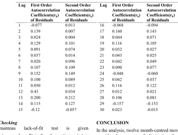
0.325 _₁0.14 _₂ the estimated

autocorrelation coefficients of residuals were obtained (Table 6) and Q1 and Q2 were computed as 34.03 and

28.62 respectively. The tests were significant and the two models fit into the production process.

However, comparing the first and second order models, the mean square error of second order is less than that of first order. That is MSE (2) = 9.107X10

9

< MSE (1) =

9.341X109 (Table 4 & 5) . Hence the model



t

t t

t

W

  

 1 0.14 2 325

.

0 is fitted for the production.

Forecasting

The autoregressive integrated moving average suitable for forecasting future production is given by

ARIMA(pdq):

e

W

t



1 t1...



p tp t



t1...



q tq

Where



_

dyt t

W

is the differenced series and





10.325, 20.148and 1and 2are to be

estimated from the autocorrelation of residuals (Table 5) using the same procedures as in equation (18). The estimates are obtained as

093 .

0

158 .

0

2

1









and

. The ARIMA model of order two suitable for forecasting future production is obtained as

e

W

t0.325 t10.148 t2 t

0 .

158

t10.093 t2

CONCLUSION

In the analysis, twelve month-centred moving average was considered as a way of eliminating the seasonal effect discovered in the series. Differenced of order twelve of the series was equally estimated to eliminate trends in order to bring the series to stationary. The autocorrelation and the partial-autocorrelation coefficients at lag thirty (30) indicated that the series is stationary. More so, two models that is autoregressive model of order one and two were fitted for the series. Autoregressive model of order two was considered to be more efficient as it has the least mean square error and is considered adequate in describing the mechanism that generated the series. For the purpose of prediction, an autoregressive integrated moving average of order two was fitted to the process.

RECOMMENDATION

For the purpose of predicting future production and process control, an autoregressive integrated moving average model of order two is therefore recommended.

REFERENCES

Allard. R. 1998. Uses of time Series analysis in Infectious Surveillance. Bulletin of World Health Organisation; 76(4): 327-33

Anderson, T. N. 1971. Statistical Analysis of time Series, Willey, New York.

Box and Jenkins, 1070. Time Series Analysis, Forecasting and Control. Holder-Day San Francisco, Düsseldorf, Johannesburg, London.

Chatfield, C. 2003. The analysis of Time Series Theory and Practice. Chapman and Hall, London.

Ernest, A. 2005. Using Autoregressive Models to predict and Monitor the number of beds occupied during a SARS outbreak in a Tertiary Hospital in Singapore. BMC Health Services Research, 11; 5: 36.

[image:6.612.124.474.81.346.2]

Priestly, M. B. 1981. Spectral analysis of Time Series: Univariate Series Vol. 1 (Probability and Mathematical Statistics) Academic Press Inc. (London) Ltd.

Table 5. Autocorrelation coefficients of residuals of fitted models

Lag First Order

Autocorrelation

Coefficients(rk)

of Residuals

Second Order Autocorrelation Coefficients(rk)

of Residuals

Lag First Order

Autocorrelation

Coefficients(rk)

of Residuals

Second Order Autocorrelation Coefficients(rk)

of Residuals

1 -0.077 0.013 16 -0.068 -0.094

2 0.139 0.007 17 0.160 0.143

3 0.024 0.004 18 0.044 0.071

4 0.129 0.101 19 0.116 0.105

5 0.091 0.074 20 0.032 0.027

6 0.037 0.014 21 0.043 0.025

7 0.020 0.096 22 0.042 0.049

8 0.107 0.109 23 0.090 0.077

9 0.152 0.149 24 -0.048 -0.060

10 0.100 0.089 25 0.042 0.037

11 0.050 0.012 26 0.116 0.122

12 0.43 0.034 27 0.012 0.021

13 0.200 0.212 28 0.106 0.081

14 0.115 0.127 29 -0.157 -0.153

15 -0.12 -0.057 30 0.023 -0.015