in Online Education
Ciara Pike-Burke, B.Sc.(Hons.), M.Res
Submitted for the Degree of Doctor of
Philosophy at Lancaster University.
This thesis is concerned with the study of sequential decision problems motivated by the challenge of selecting questions to give to students in an online educational environment. In online education there is the potential to develop personalized and adaptive learning environments, where students can receive individualized sequences of questions which update as the student is observed to be struggling or ourishing. In order to achieve this personalization, we must learn about how good each question is, while simultaneously giving students good questions. Multi-armed bandits are a pop-ular technique for sequential decision making under uncertainty. Due to their online nature and their ability to balance the trade-o between exploitation and exploration, multi-armed bandits lend themselves naturally to this problem of adaptively selecting questions in education software. However, due to the complexity of the educational problem, standard approaches to multi-armed bandits cannot be applied directly. In this thesis variants of the multi-armed bandit problem specically motivated by the issues arising in the educational domain are considered.
The rst contribution is to consider the problem of selecting questions to give to a student in a homework task, where the homework task has a xed length. Both the time it takes the student to answer each question and the benet they gain from doing so are stochastic, and so we wish to develop an algorithm which adapts to the amount of time remaining in the homework task. This is an instance of the stochastic knapsack problem and so we develop a new approach for this problem when a generative model
of item sizes and rewards is available. This algorithm is an anytime algorithm based on the optimistic planning principle. We prove that with high probability our algorithm returns a near optimal policy and bound the number of samples necessary for this.
A further problem in education is that when a student answers a question, the benet to their learning from doing so may not be evident immediately. Instead, the benet may be delayed and, when we observe an improvement in their performance, it is often unclear exactly what the contribution of each individual question was to this improvement. Hence, in an educational domain the feedback from answering questions may be delayed, but also aggregated and anonymous. The second contribution of this thesis is the study of a variant of the stochastic multi-armed bandit problem with this form of delayed, aggregated anonymous feedback. For this problem, a rarely switching algorithm is presented which is able to learn from this kind of feedback and achieve almost the same performance as a state of the art algorithm for the simpler delayed feedback bandit problem, where observations are delayed but there is no anonymity.
I have been fortunate to work with some great people during my PhD. In particular, I would like to thank my supervisors for all their help and advice. Especially, thank you to Dr Steen Grünewälder for his patience, rigor and optimism. I am grateful to have had the chance to work with someone as knowledgeable and with as much enthusiasm for research as Steen, and I have learned a lot from him. Thanks also Dr Anton Altmann for always giving me a dierent perspective on my problem during our Skype calls and for being able to solve whatever problem I was having with R. I would also like to thank Professor Jonathan Tawn and Professor David Leslie for their genuine support and encouragement (especially while I was writing up) and for the many chats about research, careers and life. Thanks also to Professor Csaba Szepesvári and Dr Shipra Agrawal for their help with the material in Chapter 5. Thank you to my examiners, Professor Nicolò Cesa-Bianchi and Dr Azadeh Khaleghi, for their helpful comments and suggestions for improving the nal version of this thesis.
I am grateful that my PhD has been funded thanks to the support of EPSRC and Sparx. I would particularly like to thank Dr Mark Dixon for his role in creating the project and everyone at Sparx (and Oxygen House) for being so welcoming and making the time I spent in Exeter so rewarding.
Thanks to all the sta and students at STOR-i for making it such a fantastic and enjoyable place to work. Special thanks must go to the rest of my year, Aaron,
Chrissy, Dan, Emma, Emma, Jack, James, Lucy, Ollie, Rebecca and Stephen for their friendship, support and willingness to watch Love Actually every Christmas. Massive thanks also to Paul and Liz for lling so many evenings with laughter, advice and good food.
Then, I got to thinking, what would I do without the girls? Thanks to Alex, Alice, Charlie, Megan, Miriam and Sarah, and Emily, Natalia and Ellie for the numerous weekends away lled with laughter, love and wine. Thank you to Adam for your kindness, humor, and support, and for always lifting me up. Thank you also to Ronan for your love and understanding.
I declare that the work in this thesis has been done by myself and has not been sub-mitted elsewhere for the award of any other degree.
Chapter 4 has been published as Pike-Burke, C. and Grünewälder, S. (2017). Opti-mistic Planning for the Stochastic Knapsack Problem. In International Conference on Articial Intelligence and Statistics.
Chapter 5 has been published as Pike-Burke, C., Agrawal, S., Szepesvári, C. and Grünewälder, S. (2018). Bandits with Delayed, Aggregated Anonymous Feedback. In International Conference on Machine Leaning.
Chapter6 has been submitted for publication as Pike-Burke, C. and Grünewälder, S. (2018). Recovering Bandits. An early version was presented at the European Work-shop on Reinforcement Leaning (2018).
The word count for this thesis is 62,073.
Ciara Pike-Burke
Abstract I
Acknowledgements III
Declaration V
Contents VI
List of Figures XII
List of Tables XIV
1 Introduction 1
1.1 Contributions . . . 4
2 Multi-Armed Bandits 7 2.1 Regret . . . 8
2.2 Popular Algorithms . . . 12
2.2.1 UCB . . . 13
2.2.2 Thompson Sampling . . . 17
2.2.3 Gittins Indicies . . . 20
2.3 Extensions . . . 22
2.3.1 Non-Stochastic Bandits . . . 22
2.3.2 Linear Bandits . . . 25
2.3.3 Gaussian Process Bandits . . . 29
2.3.4 Delayed Feedback Bandits . . . 34
2.3.5 Non-Stationary Bandits . . . 38
2.3.6 Bandits with Knapsacks . . . 45
2.3.7 Optimistic Planning . . . 46
3 Motivating Problems from Education 51 3.1 Previous Work on Using Multi-Armed Bandits in Education . . . 52
3.2 Dening the Reward . . . 56
3.3 Fixed Limit on Homework Time . . . 59
3.4 Delay in the Eect of Answering Questions . . . 61
3.5 Allowing Time between Repetitions of a Question . . . 62
4 Optimistic Planning for the Stochastic Knapsack Problem 65 4.1 Introduction . . . 65
4.1.1 Related Work . . . 68
4.1.2 Our Contribution . . . 70
4.2 Problem Formulation . . . 70
4.2.1 Planning Trees and Policies . . . 71
4.3 High Condence Bounds . . . 72
4.4 Algorithms . . . 74
4.4.1 Stochastic Optimistic Planning for Knapsacks . . . 74
4.4.2 Optimistic Stochastic Knapsacks . . . 75
4.5 -Critical Policies . . . 78
4.6 Analysis . . . 80
4.7 Experimental Results . . . 83
4.A Supplementary Material . . . 85
4.A.1 Illustration of Policies . . . 85
4.A.2 Illustration of Bounds . . . 86
4.A.3 Algorithms . . . 86
4.B Proofs of Theoretical Results . . . 87
4.B.1 Bounding the Value of a Policy . . . 87
4.B.2 Theoretical Results for Optimistic Stochastic Knapsacks (OpStoK) 94 5 Bandits with Delayed, Aggregated Anonymous Feedback 102 5.1 Introduction . . . .102
5.1.1 Our Techniques and Results . . . .105
5.1.2 Related Work . . . .107
5.1.3 Organization . . . .107
5.2 Problem Denition . . . .108
5.3 Our Algorithm . . . .110
5.4 Regret Analysis . . . .114
5.4.1 Known and Bounded Expected Delay . . . .114
5.4.2 Delay with Bounded Support . . . .116
5.4.3 Delay with Bounded Variance . . . .119
5.5 Experimental Results . . . .120
5.6 Conclusion . . . .122
5.A Supplementary Material . . . .123
5.A.1 Table of Notation . . . .123
5.A.2 Beginning and End of Phases . . . .124
5.A.3 Useful Results . . . .125
5.B Results for Known and Bounded Expected Delay . . . .126
5.B.1 High Probability Bounds . . . .126
[image:9.612.121.541.272.728.2]5.C Results for Delays with Bounded Support . . . .148
5.C.1 High Probability Bounds . . . .148
5.C.2 Regret Bounds . . . .158
5.D Results for Delay with Known and Bounded Variance and Expectation 163 5.D.1 High Probability Bounds . . . .163
5.D.2 Regret Bounds . . . .177
5.E Additional Experimental Results . . . .181
5.E.1 Increasing the Expected Delay . . . .181
5.E.2 Comparison with Vernade et al. (2017) . . . .182
5.F Naive Approach for Bounded Delays . . . .184
6 Recovering Bandits 186 6.1 Introduction . . . .186
6.2 Related Work . . . .188
6.3 Problem Denition . . . .190
6.4 Dening the Regret . . . .192
6.4.1 Full Horizon Regret . . . .192
6.4.2 Instantaneous Regret . . . .193
6.4.3 d-step Lookahead Regret . . . .193
6.5 Baseline Approach . . . .195
6.6 Gaussian Process Recovery . . . .196
6.6.1 Single Play Lookahead Regret . . . .199
6.6.2 Multiple Play Lookahead Regret . . . .200
6.6.3 Instantaneous Algorithm . . . .201
6.6.4 Bounds on the Information Gain . . . .201
6.7 Improving Computational Eciency via Optimistic Planning . . . .202
6.8 Experimental Results . . . .205
6.A Preliminaries . . . .208
6.B Theoretical Results for dRGP-UCB . . . .214
6.B.1 Non-Repeating . . . .217
6.B.2 Repeating . . . .218
6.C Theoretical Results for dRGP-TS . . . .220
6.C.1 Non-Repeating . . . .220
6.C.2 Repeating . . . .221
6.D Regret Bounds for Non-Parametric Approach . . . .221
6.E Theoretical Guarantees on Optimistic Planning Procedure . . . .223
6.F Further Experimental Results . . . .227
6.F.1 Posterior Distributions and Covariates . . . .227
6.F.2 Values of Theta in Parametric Experiments . . . .234
6.F.3 Results for Dierent Lengthscales . . . .235
7 Conclusions 238 7.1 Further Work . . . .241
7.1.1 Optimistic Planning for the Stochastic Knapsack Problem . . .242
7.1.2 Bandits with Delayed, Aggregated Anonymous Feedback . . . .243
7.1.3 Recovering Bandits . . . .245
7.1.4 Bandit Problems in Online Education . . . .247
A Useful Results and Denitions 250 A.1 Denitions . . . .250
A.2 Inequalities . . . .251
A.3 Markov Decision Processes . . . .252
A.4 Gaussian Processes and RKHS's . . . .253
A.4.1 Regression and Classication . . . .253
A.4.3 Covariance Functions . . . .255
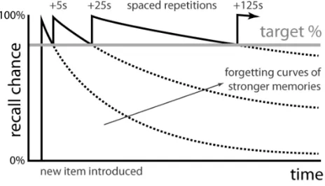
3.1 An example of a forgetting curve. . . 63
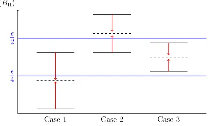
4.1 The three possible cases ofEΨ(BΠ). . . 82
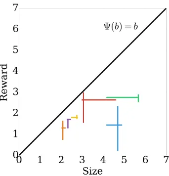
4.2 Item sizes and rewards. . . 83
4.3 Number of policies vs value. . . 84
4.4 Examples of policies in the simple 3 item, 2 sizes stochastic knapsack problem. . . 85
4.5 Example of where just looking at the optimistic policy might fail. . . . 86
5.1 The relative diculties of the dierent delayed feedback problems. . . .103
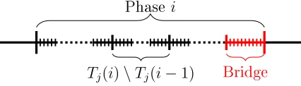
5.2 An example of phase i of our algorithm. . . .113
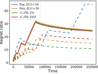
5.3 The ratios of regret of variants of our algorithm to that of QPM-D for dierent delay distributions. . . .121
5.4 A detailed example of phase i of our algorithm. . . .125
5.5 The relative increase in regret of the dierent algorithms. . . .182
5.6 The ratios of regret of variants of our algorithm to that of DUCB for dierent delay distributions. . . .182
6.1 Examples of the recovery functions. . . .189
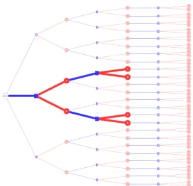
6.2 An example of ad-step lookahead tree. . . .196
6.3 The posterior recovery curves of all arms with observations indicated by crosses. . . .204
6.4 The total reward and nal depth of the lookahead tree, dN, as the
policy budget, N, increases. . . .205
6.5 Cumulative instantaneous regret for parametric setup . . . .207
6.6 dRGP-UCB with squared exponential kernel with l = 0.5. . . .228
6.7 dRGP-UCB with squared exponential kernel with l = 2. . . .229
6.8 dRGP-UCB with squared exponential kernel with l = 5. . . .230
6.9 dRGP-TS for squared exponential kernel with l = 0.5. . . .231
6.10 dRGP-TS for squared exponential kernel with l = 2. . . .232
6.11 dRGP-TS wit squared exponential kernel with l= 5. . . .233
6.12 Cumulative instantaneous regret for parametric setup withl = 2.5 . . .237
6.1 Total reward at T = 1000 for single step experiments with parametric functions . . . .205 6.2 θ values used in experiments with logistic recovery functions . . . .234
6.3 θ values used in experiments with gamma recovery functions . . . .235
6.4 Total reward at T = 1000 for single step experiments with parametric functions and l = 2.5 . . . .236 6.5 Total reward at T = 1000 for single step experiments with parametric
functions and l = 7.5 . . . .236
Introduction
The world of education is changing. With the development of the internet and smart-phones, people across the world are increasingly able to access encyclopedias worth of knowledge from their pockets. This has dramatically changed how people learn and develop new skills. One example of this is the development of Massive Open Online Courses (MOOCs), e.g. EdX www.edx.org and coursera www.coursera.org,
and other large online courses which mean that anyone can sign up for courses oered by top institutions and follow these courses online, using online quizzes to test their knowledge. On a smaller scale, there are now a multitude of educational games and apps available online where students can learn or consolidate skills while having fun. Even in a traditional education environment, teaching is now being aided by the use of online quizzes and tests, which allow teachers to track the performance of their students in realtime. All this contributes to a new, more online, way of learning.
One of the most exciting aspects of online education is the potential for personal-izing learning. This means that each student can be given individual tasks specically tailored to their strengths and weaknesses. The benets of this would be enormous, struggling students would have the time to revise key concepts and learn at their own pace, whereas students who are excelling can be pushed further and their knowledge
deepened. Moreover, these online education systems also have the potential to adapt to how the student is getting on in a specic task, noticing right away if a student is struggling and taking direct action to help them. The challenge is how to achieve this. How do we decide which questions to give to the student when we do not know a priori how benecial each one is? And how do we use the limited data we observe about the students to improve our future decisions?
Sequential decision models are a way of mathematically formalizing the concept of making a decision and using feedback on the outcome of that decision to inform future decisions. Within this area, algorithms for the multi-armed bandit problem will be particularly useful. The multi-armed bandit problem gets its name from the classical casino analogy of choosing which one armed bandit (slot machine) to play in order to maximize the payout, when the payout of each slot machine is stochastic with unknown expectation. In order to maximize their total winnings, a player must decide whether to explore their options, gathering more information about the slot machines, or exploit their current knowledge to select one which currently looks good. In recent years algorithms for multi-armed bandits have been developed and applied to settings such as online advertising, website optimization and recommendation systems to great success. One reason for this success is their ability to expertly and accurately balance the trade-o between wanting to explore and learn about the eectiveness of dierent actions and wanting to exploit the current knowledge and take the best action. This is similar to the challenge faced when trying to decide which questions to give to a student in an online education setting. However, the complexities of the educational domain mean that standard algorithms for the multi-armed bandit problem cannot directly be applied. The aim of this thesis is to investigate multi-armed bandit models inspired by the problem of selecting personalized questions in online education.
The work of this thesis has been carried out in collaboration with Sparx, an educa-tion research company. Since their foundaeduca-tion, Sparx have been gathering data on student performance in a series of online exercises accessed via their app. The app is incorporated into a traditional teaching environment and is designed to aid the teachers as well as the students. Once a teacher introduces a topic, the students will work through some exercises on the app, both in class and at home. As they do so, data will be obtained tracking their progress. The data consists of logging student interaction with the online platform and, as such, may be a lot more detailed than that gathered in a traditional schooling environment. Sparx's long term aim is to be able to use this extra information to improve students' experience and attainment. The aim of this particular work is to develop sequential decision making algorithms that are able to learn from this detailed feedback and suggest good questions to give to the students.
In this thesis, the focus will be on the statistical and mathematical foundations of multi-armed bandit algorithms motivated by this problem of suggesting questions to students in an online education environment. There are many challenges in the educational domain which make applying the standard algorithms for multi-armed bandits dicult. The three main challenges that have motivated the methodological work in this thesis are the following. Firstly, when we are setting homework tasks, there is a limit on the amount of time each homework can take, so we need to develop approaches that can handle this short horizon and adapt to the time remaining in the homework. Furthermore, when a student answers a question, the benet they gain from doing so is not immediate, but instead is only observed as an aggregate sometime after answering the question. Lastly, the benet to a student of answering a question will not be constant over time, it will most likely depend on how long it has been since they answered similar questions.
1.1 Contributions
This thesis studies sequential decision problems which are motivated by the challenge of selecting questions to give to students in an online education environment. In Chapter2 we will introduce the multi-armed bandit problem and give an overview of some related work on algorithms and extensions to the classical problem. In Chapter3 we will discuss existing work on using multi-armed bandits in online education do-mains and give further details of the specic problems in online education which have motivated the work in this thesis. The main contributions of this thesis are method-ological developments in the eld of multi-armed bandits. These will be presented in Chapters 4Chapter 6. The work in each of these chapters has been submitted for publication as a standalone paper, and as such there may be some repetition of material. We outline below the main technical contributions of each of these chapters.
Chapter 4: Optimistic Planning for the Stochastic Knapsack
Problem
The stochastic knapsack problem is a stochastic resource allocation problem that arises frequently and yet is exceptionally hard to solve. We derive and study an opti-mistic planning algorithm specically designed for the stochastic knapsack problem. Unlike other optimistic planning algorithms for Markov Decision Processes (MDPs), our algorithm, OpStoK, avoids the use of discounting and is adaptive to the amount of resources available. We achieve this behavior by means of a concentration inequal-ity that simultaneously applies to capacinequal-ity and reward estimates. Crucially, we are able to guarantee that the aforementioned condence regions hold collectively over all time steps by an application of Doob's inequality. We demonstrate that the method returns an -optimal solution to the stochastic knapsack problem with high
guarantees for the stochastic knapsack problem. Furthermore, our algorithm is an anytime algorithm and will return a good solution even if stopped prematurely. This is particularly important given the diculty of the problem. We also provide theo-retical conditions to guarantee OpStoK does not expand all policies and demonstrate favorable performance in a simple experimental setting.
The work in this chapter appeared as: Pike-Burke, C. and Grünewälder, S. (2017). Optimistic Planning for the Stochastic Knapsack Problem. In International Confer-ence on Articial IntelligConfer-ence and Statistics.
Chapter 5: Bandits with Delayed, Aggregated Anonymous
Feed-back
We study a variant of the stochasticK-armed bandit problem, which we call bandits
with delayed, aggregated anonymous feedback. In this problem, when the player pulls an arm, a reward is generated, however it is not immediately observed. Instead, at the end of each round the player observes only the sum of a number of previously generated rewards which happen to arrive in the given round. The rewards are stochastically delayed and due to the aggregated nature of the observations, the information of which arm led to a particular reward is lost. The question is what is the cost of the information loss due to this delayed, aggregated anonymous feedback? Previous works have studied bandits with stochastic, non-anonymous delays and found that the regret increases only by an additive factor relating to the expected delay. In Chapter5, we show that this additive regret increase can be maintained in the harder delayed, aggregated anonymous feedback setting when the expected delay (or a bound on it) is known. We provide an algorithm that matches the worst case regret of the non-anonymous problem exactly when the delays are bounded, and up to logarithmic factors or an additive variance term for unbounded delays.
C. and Grünewälder, S. (2018). Bandits with Delayed, Aggregated Anonymous Feed-back. In International Conference on Machine Leaning.
Chapter 6: Recovering Bandits
The recovering bandits problem is a variant of the non-stationary stochastic mutli-armed bandit problem designed to capture the eect of the time between plays on the reward of a given arm. In many scenarios such as product recommendation, the benet of suggesting a product will depend on how long it has been since it was last suggested. This is captured in recovering bandits where, the expected reward of each arm changes depending on the time since the arm was last played according to some unknown recovery function. Under the assumption that the recovery functions are sampled from a Gaussian process, we present and analyze two algorithms for the recovering bandits problem. Furthermore, we show how their performance can be improved by allowing them to lookahead and select good sequences of actions. Finally, we demonstrate the experimental performance of our algorithms and present an approximation based on optimistic planning to improve computational eciency at little cost to accuracy.
Multi-Armed Bandits
The multi-armed bandit problem is a classical sequential decision problem that has been studied for many years (for example by Thompson (1933); Lai and Robbins (1985); Auer et al. (2002a); Gittins et al. (2011); Bubeck and Cesa-Bianchi (2012); Lattimore and Szepesvári(2018)). It gets its name from the fact that in its simplest form it can be expressed using an analogy to slot machines (or one-armed bandits) in a casino. Assume that a player is faced with a row of slot machines, or arms, and that each slot machine has a dierent probability distribution governing the payo it generates when it is played. We call the payo the player receives the reward from playing an arm. All the reward distributions are unknown to the player, whose aim is to play the slot machines that will maximize the total reward. The player's task is then to choose between playing arms that they already know produce a high reward, or trying alternative arms about which they have less information, but whose reward could be high. The player must therefore decide how to trade-o between exploiting good arms to maximize their immediate reward and exploring other arms to gather information about their performance in order to potentially improve future rewards.
Formally, we dene the stochastic K-armed bandit as follows. We assume that
there areK arms (or actions, the two terms will be used interchangeably in this
sis) in a set A, and associated with every arm 1 ≤ j ≤ K is an underlying reward
distribution νj. Whenever an arm j is played a stochastic reward is generated
in-dependently from the underlying distribution νj and presented to the player. The
multi-armed bandit problem proceeds in rounds and, in each round, the player selects an arm and then receives a reward from the underlying reward distribution of that arm. The player can then use the previously observed rewards to inform future de-cisions about which arms to play. We dene the horizon, T, as the total number of
plays of the bandit game. The game can be summarized in the following sequence. Beginning with an empty history, H0 =∅, at each time stept = 1, . . . , T, the player,
1. Selects an arm Jt ∈ {1, . . . , K}, possibly using the historyHt−1
2. Receives an observation Xt,Jt ∼νJt
3. Adds the pair {Jt, Xt,Jt} to the history, Ht=Ht−1∪ {Jt, Xt,Jt}.
The player's aim is to select the actions that will maximize their total reward overT
time steps.
It is typically necessary to make some assumptions about the reward distributions,
νj, in order to construct a tractable algorithm for the multi-armed bandit problem.
Generally, it is assumed that the rewards of all arms are independent and that all arms
j = 1, . . . , K have a nite expectations µ1, . . . , µK (so E[X1,j] = µj for X1,j ∼ νj).
In some cases, it is assumed that the reward distribution is from a particular family of distributions. Otherwise, it is assumed that the reward distributions are (λ
-)sub-Gaussian (see Appendix A.1) or bounded, often in[0,1].
2.1 Regret
was used and the aim was to maximize the expected discounted reward. However, recently an alternative performance measure has been considered. In particular, the performance of an algorithm for the multi-armed bandit problem is typically measured in terms of its (cumulative) regret. The cumulative regret up to horizonT,RT, is the
total dierence in the reward that could have been obtained by repeatedly playing the optimal arm and the reward that was actually obtained by the arms played. We will mostly be interested in the expected regret of an algorithm, where the expectation is taken over the actions taken (note that the actions may be random variables since they can depend on the past observations). Specically, let µ∗ = max1≤j≤Kµj be
the maximum expected reward of any arm. Clearly the best possible algorithm will constantly play this arm for all T rounds. We dene the regret as the dierence in
expected cumulative reward between this oracle and the arms J1, . . . , JT chosen by
the algorithm. In particular, we dene the expected cumulative regret up to horizon
T as,
E[RT] = T
X
t=1
E[µ∗−µJt].
The aim of a bandit algorithm is to select arms Jt in order to minimize this expected
regret. Note that this is essentially equivalent to maximizing the expected cumulative reward of the algorithm.
The problem dependent regret of a bandit algorithm depends on the specics of the problem instance we are considering. For a particular setA of actions numbered
1 to K, the problem dependent regret will typically depend on the means, µj, of the
actions. For any armj 6=j∗, let∆j =µ∗−µj be the sub-optimality gap of arm j and
for any arm j, and let Nj(T) be the random number of times armj has been played
up to horizon T. Then the expected regret can be expressed as,
E[RT] = K
X
j=1;j6=j∗
∆jE[Nj(T)]
Using this in their seminal paper,Lai and Robbins (1985) proved the following lower bound on the problem dependent regret of any bandit algorithm. Specically, under some mild assumptions on the reward distributions (see (Lai and Robbins, 1985) for details), it was shown that the regret of any algorithm for the multi-armed bandit problem must satisfy,
lim inf
T→∞
E[RT]
logT ≥
K
X
j=1;j6=j∗
∆j
KL(νj, νj∗) (2.1)
whereKL(νj, νj∗)represents the Kullback-Leibler divergence between the reward
dis-tribution of armj and that of the optimal arm (see Appendix A.1). This means that
in this problem setting, no algorithm can achieve a smaller problem dependent rate of regret. Hence, the aim is often to construct algorithms that can achieve problem dependent regret of this order.
Sometimes it is not desirable to bound the regret of a bandit algorithm for a particular problem instance. In practice, the expected rewards, µj's, of each arm are
on the problem independent regret of any bandit algorithm. Particularly, for any algorithm, there exists a problem instance where
E[RT]≥
1 20min{
√
KT , T}. (2.2)
This is a bound on the regret of the algorithm in the worst possible case (in fact, it is derived for the adversarial bandit problem, see Section 2.3.1) and so it is natural that it is larger than the problem dependent regret bound.
The above denitions of regret have all assumed a frequentist representation of the problem. In some cases it is desirable to take a Bayesian approach (see e.g. Gelman et al.(2013) for an introduction to Bayesian reasoning). Here, any parameters of the reward distribution are assumed to be random variables and a prior distribution is placed on them. This induces a prior distribution over theµj's for all arms1≤j ≤K.
In this case, the regret denition changes and we consider the Bayesian regret. In the Bayesian regret, the expectation is taken over this prior distribution as well as the arms selected. Hence, we dene the cumulative Bayesian regret up to horizonT as,
E[RBT] = T
X
t=1
E[µ∗−µJt] =
T
X
t=1
E[E[µ∗−µJt|µ1. . . µK]].
Bubeck and Liu (2013) state that the lower bound of (2.2) also holds for Bayesian regret when the rewards are in[0,1]. This means that in the Bayesian setting we we can always nd a prior distribution such that the Bayesian regret satises E[RBT] =
Ω(√KT). In a slightly dierent setting where the rewards are discounted, it is possible to design algorithms which asymptotically match the expected cumulative discounted reward (where the expectation is taken with respect to the prior as well) of the optimal strategy (see Section2.2.3 for details).
The challenge is therefore to develop algorithms for the multi-armed bandit problem that achieve these rates of regret. Furthermore, it is desirable to develop algorithms which exhibit strong nite time regret as well as asymptotically having low regret. Finite time regret is the regret up to a xed horizonT and is more informative about
the real life performance of the algorithm. In the following section (Section 2.2), we detail some of the key algorithmic developments that have lead to (near) optimal algorithms for the stochastic multi-armed bandit problem.
2.2 Popular Algorithms
2.2.1 UCB
The use of optimistic estimates or Upper Condence Bounds (UCBs) for the multi-armed bandit problem stems from the seminal work ofLai and Robbins(1985). Intu-itively, the idea behind the upper condence bound approach is to use an optimistic estimate of the expected reward of each arm given the information available. Then, playing the arm with the largest optimistic estimate will lead to selecting arms which either have high reward or are poorly estimated, in which case they are worth ex-ploring more. The condence bounds presented in (Lai and Robbins, 1985) relied on the entire history of rewards of all arms and as such were dicult to compute. A simpler algorithm was proposed by Agrawal (1995) who provided an asymptotic analysis. This was later adapted by Auer et al. (2002a), who provided a nite time analysis of the regret of this algorithm, and several other related algorithms.
The UCB1 algorithm from (Auer et al.,2002a) constructs upper condence bounds around the sample mean of the reward of each arm in a way that guarantees that the true mean of the arm is less than the upper condence bound with high probability. These are constructed using Hoeding's inequality (see Appendix A.2) and hold for any reward distribution bounded in [0,1]. For any arm j which has been played nj
times, let X¯
j be the sample mean of these nj observations, then, with probability
greater that1−δ,
µj ≤X¯j +
s
log(1/δ) 2nj
.
This is used in the construction of the upper condence bounds of the UCB1 algo-rithm. In particular, the UCB1 algorithm proceeds by playing each arm once to guar-antee that the initial sample means exist, and then at each time stept=K+ 1, . . . , T,
it selects arm,
Jt = arg max
1≤j≤K
¯
Xj,t+
s
log(t) 2Nj(t)
game and X¯
j,t = Nj(t) s=1Xs,JsI{Js=j} is the sample mean of these observations. Note that the only knowledge the UCB1 algorithm has about the reward distribution is that the arms are independent and the rewards are bounded in[0,1].
Auer et al. (2002a) showed that the problem dependent regret of UCB1 satises,
E[RT]≤8 K
X
j=1
log(T) ∆j
+ (1 +π2/3)
K
X
j=1
∆j.
This has the same log(T) dependence on the horizon T as seen in the lower bound
(2.1). Moreover, for Normal distributions with means µ∗ and µj and unit variances,
the KL divergence simplies to∆2j in which case the lower bound in (2.1) is matched exactly by the dominant term of this regret bound. However, for alternative reward distributions, KL(νj, νj∗) 6= ∆2j and so this upper bound does not match the lower
bound in (2.1) exactly. The proof of this regret bound relies on bounding E[Nj(T)],
the expected number of times any sub-optimal arm is played by the algorithm. It can be shown that if Nj(T) > 8log(∆2T)
j , then the condence term for arm
j is smaller
than∆j/2, and so the only way armj can be played again is if the condence bounds
on arm j or the optimal arm fail. By Hoeding's inequality, this happens with low
probability. Hence the main contribution of arm j to the regret is from these rst
plays when the algorithm is learning about the arm and this is bounded by∆j8log(∆2T)
j . This gives the result. From this problem dependent regret bound, it is easy to show that the problem independent regret of UCB1 satises,
E[RT]≤O(
p
KTlog(T)). (2.3)
This matches the order of the lower bound in (2.2) up to a p
the problem dependent regret to nd the worst case value of ∆ (see for example, (Lattimore and Szepesvári,2018)). This gives the problem independent regret bound. This value of ∆ represents the sub-optimality gap that is hardest for the algorithm to deal with.
While UCB1 is a simple and intuitive algorithm that enjoys theoretical guarantees on the regret that almost match the lower bounds in (2.1) and (2.2), considerable eort has been invested in constructing UCB approaches for the multi-armed bandit problem which have tighter regret bounds. One of the most important of these, the KL-UCB algorithm of Cappé et al. (2013), aims to recover the KL divergence term in the denominator of (2.1) and thus focuses on problem dependent regret. For a one parameter exponential family reward distribution which can be parameterized by the mean, their approach is to to construct a pseudo upper condence bound for each arm by selecting the parameter that will maximize the expected reward while still being close to the sample mean in KL distance. Specically, let d(µ, µ0) be the KL-divergence between the particular exponential family distribution of interest when the mean parameters areµ∈Θand µ0 ∈Θ(andΘis the parameter set). In the KL-UCB algorithm, each arm is played once to begin with, then at time t=K+ 1, . . . , T, we
play arm
Jt= arg max
1≤j≤K
sup
µ∈Θ;d( ¯Xj,t, µ)≤
log(t) + 3 log(log(t))
Nj(t)
.
Cappé et al.(2013) show that the regret of this algorithm satises,
E[RT]≤
K
X
j=1
∆j
log(T)
d(µj, µ∗)
(1 +o(1)).
Hence, the problem dependent regret of KL-UCB matches the lower bound in (2.1) up to lower order terms. Note that using Pinsker's inequality to bound d(µj, µ∗) ≥
1
2(µj −µ
∗)2 = 1 2∆
2
independent regret bound ofO( KTlog(T))for KL-UCB, the same as UCB1. Cappé et al.(2013) also provide a version of the algorithm for distributions which are not one parameter exponential family. However, note that, in all cases, in order to calculate the selection criteria, it is necessary to be able to calculate the KL-divergence and this requires knowledge of the reward distributions, which is not required for UCB1.
The problem independent regret of UCB1 in (2.3) suers from an additional
p
log(T) term compared to the lower bound in (2.2). There have been several ap-proaches designed to remove this term. The rst, the so-called Improved-UCB algo-rithm of Auer and Ortner (2010), is an example of a rarely switching algorithm. It runs in phases and in each phase it plays each active arm consecutively and then, at the end of a phase, an active arm is eliminated if it is clearly suboptimal. Specif-ically, in every phase i, the algorithm maintains a tolerance gap ∆˜i and plays each
active arm until the total number of times it has been played is ni =
2 log(T∆˜2
i)
˜ ∆2
i
. Then an arm is eliminated if its estimated mean reward is further than ∆˜
i from the
best estimated mean reward, and the tolerance gap is reduced, ∆˜
i+1 = ˜∆i/2. The
regret analysis of this algorithm again uses Hoeding's inequality (but this time to get condence bounds that hold with probability greater than1− 1
T∆˜2
i in each phase
i) to bound the probability of erroneously eliminating arms. This leads to problem
dependent regretE[RT]≤PKj=1
Clog(T∆2
j)
∆j for some constantC > 1. This corresponds to problem independent regret of
E[RT]≤O(
p
KTlog(K)).
This is an improvement over the worst case regret of UCB1 by replacing p
log(T) with p
log(K). However, it is still loose by plog(K).
plays arm
Jt= arg max
1≤j≤K
¯
Xj,t+
s
max{log(KNT
j(t)),0}
Nj(t)
.
This leads to problem dependent regret ofE[RT]≤CK
PK
j=1
max{log(T∆2
j/K),1}
∆j which corresponds to a problem independent regret bound of
E[RT]≤O(
√
KT),
matching the optimal rate indicated by (2.2).
2.2.2 Thompson Sampling
One of the earliest instances of the multi-armed bandit problem appeared in (Thomp-son, 1933) in the context of clinical trials. The proposed algorithm, now known as Thompson sampling, is very popular due to its intuitiveness, ease of implementation and strong experimental performance. It is a Bayesian approach and so begins with placing a prior distribution over the parameters of the reward distribution of each arm. Let θj be the parameters of the reward distribution over arm j and let r(θ)
give the expected reward as a function the parametersθ (which is common across all
arms). Let π(θj) be the prior placed on the parameters of arm j. Then, under the
assumption that the family of reward distributions is known, the posterior distribu-tion of the parameters can be obtained by using the likelihood of the observadistribu-tions of arm j (see (Gelman et al., 2013) for further details). For any arm j and time t, let πt(θj) denote the posterior distribution ofθj at time t, using the Nj(t)previously
ob-served samples from the reward distribution of armj. Then the Thompson sampling
algorithm proceeds as follows. At time t,
1. For all arms 1≤j ≤K, sample θ˜j ∼πt(θj)
Note that since we have a prior distribution over each θj, we do not need an
initial-ization step as in the UCB approaches. It can be shown that at time t, the above
procedure is equivalent to playing each arm with the posterior probability that it is optimal. If the reward distributions admit a conjugate prior (e.g. exponential fam-ily distributions), the posterior distributions of the reward parameters can be easfam-ily computed. If not, alternative methods such as MCMC (see e.g. (Gilks et al., 1995)) may need to be used in order to obtain samples from the posterior.
The strong empirical performance of Thompson sampling was demonstrated in (May and Leslie, 2011; Chapelle and Li, 2011) where it was shown to outperform the UCB approach in various experiments. May et al. (2012) proved asymptotic results on the performance of Thompson Sampling for general reward distributions. Theoretical regret bounds for Thompson sampling were given in (Agrawal and Goyal, 2012) and (Kaufmann et al.,2012b). These results consider the Beta-Bernoulli bandit problem, where the prior on the expected reward of each arm is a Beta distribution and the observations of each arm are Bernoulli, leading to a conjugate Beta posterior. However, as discussed in (Agrawal and Goyal, 2012), this can be extended to other reward distributions taking values in [0,1] by rst observing the random reward Xj,t
and then performing a Bernoulli trial with success probability Xj,t and updating the
posterior distribution of a pseudo parameterθj for these Bernoulli trials for armj.
Kaufmann et al. (2012b) mainly considered the problem dependent regret and proved that for any >0, the expected regret of Thompson Sampling satises,
E[RT]≤(1 +) K
X
j=1
∆j(log(T) log(log(T)))
KL(µj, µ∗)
+C(,µ).
whereC is a constant depending onandµ= (µ1, . . . , µK). This almost matches the
prove a slightly dierent problem dependent regret bound and also show that the problem independent regret of Thompson Sampling satises,
E[RT]≤O(
p
KTlog(T))
for the Beta-Bernoulli bandit problem. This is the same problem independent regret rate as UCB1 (Auer et al., 2002a) and has an additionalp
log(T)term compared to the lower bound in (2.2). These results for Beta-Bernoulli bandits were extended in (Korda et al., 2013) to cover reward distributions in the one-parameter exponential family and in (Agrawal and Goyal, 2013a) to consider Gaussian distributions, and similar results were shown.
All the above theoretical results focused on the frequentist regret (where the mean rewards are xed and the expectation is only taken over the arms chosen). However, since Thompson sampling is a Bayesian procedure, is also makes sense to consider the Bayesian regret. Theoretical regret guarantees on the Bayesian regret of Thompson Sampling were obtained byRusso and Van Roy (2014). Here, they were able to relate the Bayesian regret of Thompson sampling to that of a UCB approach, and using results on the performance of various UCB strategies, they obtained Bayesian regret bounds for a wide variety of dierent settings. For nitely many arms, they show that the Bayesian regret isO(pKTlog(T)). This was improved in (Bubeck and Liu,2013) where it was shown that the Bayesian regret of Thompson sampling isO(√KT).
There have also been variations of the Thompson Sampling algorithm considered in the literature. The Optimistic Bayesian Sampling algorithm of May et al. (2012) aims to combine Thompson sampling with the optimistic principle underpinning the UCB strategies. Here, at each time step, t, after sampling θ˜j from the posterior of
of the sum of rewards from their algorithm to the sum of optimal reward will tend to 1. Another approach aimed at combining Bayesian and optimistic strategies is the Bayes UCB algorithm ofKaufmann et al. (2012a). This approach uses the quan-tiles of the posterior distribution as upper condence bounds and then proceeds as a standard UCB algorithm. They show that this approach achieves problem dependent frequentist regret for Bernoulli rewards of
E[RT]≤ K
X
j=1
(1 +)∆j
KL(µj, µ∗j)
log(T) +c(log(T))
for >0wherec is some constant depending on. They also show that, for Bernoulli
rewards, the index they use is equivalent to the index used in the KL-UCB algorithm.
2.2.3 Gittins Indicies
A dierent Bayesian approach to the multi-armed bandit problem is the Gittins Index approach (Gittins et al., 2011; Gittins, 1979). In this framework, the multi-armed bandit problem is represented as a (semi) Markov decision process (see AppendixA.3) where the state is the current posterior distribution over the reward parameters of each arm and the actions are the set of arms in the bandit problem. It is assumed that the state of each arm evolves according to an independent Markov chain with transition density D. At each time t, the player observes the states of each arm j, Sj(t), and selects an action. If the action chosen at timetis armJt, the player receives
a reward r(SJt(t)) and then the states are updated so that Sj(t+ 1) = Sj(t) for all
j 6=Jt and SJt(t+ 1) =D(SJt(t)).
In this setting, the aim is normally to maximize the expected total discounted reward,E
PT
t=1γtr(SJt(t))
that dynamic programming will nd the optimal policy (Bellman, 1956). However, in a MDP representation of the bandit problem, the state space is very large and so such a dynamic programming solution would not be computationally tractable. Despite this, Gittins (1979) (see (Gittins et al., 2011) for alternative proofs) showed that there exists an optimal index style policy that denes an index for each arm independently. Playing arms with the largest such index at each time step maximizes the total expected discounted reward of a policy. This is the so-called Gittins index policy.
The Gittins index policy consists of playing the arm from a given state with highest Gittins index. The Gittins index of arm j from initial state s is dened as,
G(j, s) = sup
τ >0
E
Pτ−1
t=0 γ
tr(S j(t))
Sj(0) =s
E
Pτ−1
t=0 γt
Sj(0) =s
,
where Sj(t) = D(Sj(t−1)). Note that this can be intuitively interpreted for each
arm as the largest cost the player is willing to pay to receive at least one more reward from that process (Lattimore and Szepesvári, 2018). It is then shown that playing arm Jt = arg max1≤j≤KG(j, Sj(t)) at time t maximizes the cumulative discounted
expected reward, E
P∞
t=1γ
tr(S Jt(t))
. Finite time regret guarantees of the Gittins index policy were provided by Lattimore (2016).
problems. Furthermore, for most of the problems studied here, using Gittins indicies would involve including an articial discount factor which may not be appropriate.
2.3 Extensions
The multi-armed bandit problem as presented above is an interesting problem for which several algorithms have been developed. However, it can be argued that in its present form it is too simple for many applications. Consequently, there have been numerous extensions to the standard stochastic K-armed bandit problem to make
it more appropriate in many practical applications. We detail here some of these extensions which are most relevant to the work in this thesis.
2.3.1 Non-Stochastic Bandits
Another version of the bandit problem that has been studied in the literature is the non-stochastic or adversarial bandit problem. This problem was rst introduced by Auer et al. (1995) and removes several of the assumptions underlying the stochastic multi-armed bandit problem. Specically, in the adversarial bandits problem, it is no longer assumed that the rewards are sampled from an underlying reward distribution, nor that they are even random variables. Instead, they are assumed to lie in [0,1] and to be generated by an `adversary'. At each timet, the adversary selects a vector
xt = (x1,t, . . . , xK,t)T of rewards in [0,1]K. Then, if the player plays arm Jt at time
The performance of an algorithm for the adversarial bandits problem is again measured in terms of its regret. However, the denition of regret here diers slightly from in the stochastic bandit problem. Since the adversary choses a vector of rewards at each time step, the best arm is constantly changing, however, the regret is dened with respect to the best constant arm, that is arg max1≤j≤KPT
t=1xj,t. Note that by
Arora et al.(2012) this is more appropriate since sub-linear regret with respect to the best sequence of actions is not possible. We are also often interested in the worst case regret which is taken over all possible action choices of the adversary. Hence, in the adversarialK-armed bandit problem, the regret is dened as,
E[RaT] = max x1,...,xT
max
1≤j≤K T
X
t=1
xj,t−E
T X
t=1 xJt,t
,
where the expectation is taken over the potential randomness of the choice of actions. The worst case lower bound on the regret in (2.2) was proved for the adversarial bandits problem, and so also holds in this case.
As mentioned previously, randomized strategies will generally outperform deter-ministic ones in the adversarial bandits problem. Interestingly, this means that of-ten algorithms for the stochastic bandits problem perform poorly in the adversarial problem. Hence specic strategies have been developed for the adversarial bandits problem. The rst such algorithm to be proposed was the EXP3 algorithm of Auer et al. (1995), which is based on the Hedge algorithm of Freund and Schapire (1997). At each time step t, EXP3 plays arm j with probability Pj,t. These probabilities
are calculated using exponential weighting of importance sampling estimators of each arm's reward. Specically, let Sˆ
j,t =
Pt
n=1
I{Jn=j}xj,n
Pj,n for all arms j, then at time t, arm j is played with probability,
Pj,t = (1−η)
exp{ηSˆj,t/K}
PK
j=1exp{ηSˆj,t/K}
+ η
whereηis a tuning parameter used to control how quickly we want to stop exploring.
When η=
q
Klog(K)
(e−1)T , the regret of EXP3 is bounded by,
E[RaT]≤2
p
(e−1)KTlog(K).
This matches the lower bound in (2.2) up to logarithmic factors.
There have also been numerous variants of the EXP3 algorithm and dierent ap-proaches proposed in the literature. These include algorithms designed to remove the logarithmic terms (Audibert and Bubeck,2009), algorithms with high probability regret guarantees (Neu, 2015), or general algorithms for both stochastic and adver-sarial bandits (Auer and Chiang, 2016; Seldin and Lugosi, 2017) among others. Of particular relevance to us is the `bandits with expert advice' problem and the EXP4 algorithm of Auer et al. (1995). In the bandits with expert advice problem, at each time t, the player is presented with N probability vectors over the arms, each
rep-resenting a dierent expert's opinion of which arm to play. The player can then use this expert advice to inuence their choice of which action to take. Here, the regret is dened with respect to the expected reward of the best expert. Formally, if the beliefs of expertsi= 1, . . . , N at timet= 1, . . . , T are represented by the probability vectors ξ1(t), . . . ,ξN(t) and xt is the vector of the rewards of each arm, then the regret is
dened as
E[ReT] = max
1≤i≤N T
X
t=1
ξi(t)Txt−E
T X
t=1 xJt,t
,
when the player plays actions J1, . . . , JT. The EXP4 algorithm of Auer et al. (1995)
is a modication of EXP3 to this setting. For some tuning parameter γ ∈ (0,1], at each time step t = 1, . . . , T, the learner recieves the expert advice vectors and then
plays arm j with probability
Pj,t = (1−γ)
PN
i=1wi(t)ξ
(j)
i (t)
PN
i=1wi(t)
+ γ
where wi(t) is the weight given to expert i at time t and is dened iteratively by
wi(1) = 1,wi(t+ 1) =wi(t) exp(γξi(t)
Tyi(t)
K )wherey
(j)
i =I{Jt =j}Pxj,t
j,t and superscript (j) is used to denote the jth element of a vector. Under the assumption that the
family of experts contains the uniform expert, Auer et al. (1995) proved that the regret of the EXP4 algorithm in the bandits with experts problem is bounded by
E[ReT]≤(e−1)γmax1≤i≤N
PT
t=1ξi(t)Txt+Klog(γ N).
Since the adversarial bandit problem removes many assumptions about the reward generating process, it can often be used as a baseline in variants of the stochastic ban-dit problem which change the assumptions on the reward generating process (although sometimes the regret denition will be dierent). For example, when the rewards are stochastic but the distributions can change over time, adversarial bandit algorithms can be used as a baseline for comparison. It is mainly for this purpose that adversarial bandits will be considered in this thesis.
2.3.2 Linear Bandits
In all of the bandit models so far described, it has been assumed that there are only nitely many arms and the regret bounds presented scale with the number of arms. However, often we are in settings where we have a very large, or possibly innite, number of arms. In this case it is desirable to develop algorithms that scale better. Clearly, this will be impossible if all the arms are still assumed to be independent and there is no information shared between them. Therefore, it is necessary to make some assumptions on the structure and correlation between the arms. The simplest such assumption is that each action can be represented as a d dimensional feature vector,
and that the expected reward is the inner product of this feature vector with some unknown d dimensional parameter vector, θ∗, common to all actions. This setting is
formalized in the linear bandits problem.
an actionXt ∈ Xt ⊂R from a possibly changing set of ddimensional feature vectors
Xt. The player then receives reward
Yt=hXt, θ∗i+t,
wheret is conditionally R-sub-Gaussian noise (see AppendixA.1) andθ∗ ∈Θ⊂Rd.
Note that it is assumed that the player has knowledge of the feature vectors of all actions X ∈ Xt and that it is the parameter θ∗ which is unknown (although Θ will
typically be known). The performance of an algorithm for the linear bandits problem is again typically measured in terms of it's regret. In this case, the regret up to horizon
T is,
RT =
T
X
t=1
max
X∈Xt
hX, θ∗i −
T
X
t=1
hXt, θ∗i.
Note that this is not the expected regret and many approaches for linear bandits will give high probability regret bounds. As in the stochastic K-armed bandit problem,
there have been algorithms developed for linear bandits based on both the upper condence bound and Thompson sampling approaches. Before discussing these, it is worth considering lower bounds on the regret.
Multiple lower bounds on the regret in the linear bandits problem have been presented under dierent assumptions aboutXt. Firstly, if Xt =X = {(x1, . . . , xd) :
x2
1+x22 =x23+x24 =· · ·=x2d−1+x2d= 1} is the Cartesian product of d/2 circles, with
θ∗ restricted so that rewards lie in {−1,1}, then Dani et al. (2008) showed that the
regret must be Ω(d√T). If the action set is a hypercube, that is Xt =X = [−1,1]d,
andΘ ={−1/√T ,1/√T}d, the regret must also satisfy
E[RT] = Ω(d
√
T)(Lattimore and Szepesvári, 2018). Additionally, when d ≤ 2T and the action set is a sphere
Xt = X = {x ∈ Rd : kxk2 = 1}, then there exists a θ ∈ Rd with kθk2 = d/
√
T
such thatE[RT] = Ω(d
√
Asymptotic lower bounds for linear bandits with nite action spaces were proven in (Lattimore and Szepesvari, 2017).
In the upper condence bound approaches for linear bandits, the general idea is to construct high probability bounds on θ∗. In linear bandits, these upper condence
bounds on θ∗ are constructed by estimating θ∗ (often by regularized least squares)
using all past observations(X1, Y1), . . . ,(Xt−1, Yt−1) and then building condence
el-lipsoids around this estimate which contain θ∗ with high probability. Then, at each
time step t, the action Xt which maximizes the inner product with some θ in the
condence set Ct−1, is selected, i.e.,
select ( ˜Xt,θ˜t) = arg max
(x,θ)∈Xt×Ct−1
hx, θi then play, Xt= ˜Xt.
The key issue when dening condence sets for this problem is to deal with the depen-dencies between the covariates. The rst optimistic approach to the linear bandits problem was in (Auer, 2002) where the dependencies were dealt with theoretically by using a wrapper algorithm to divide observations into sets of almost independent observations. A similar approach was taken in (Chu et al.,2011) and (Li et al.,2010). Dani et al. (2008) use a more sophisticated martingale argument to deal with the dependencies, through which they are able to obtain a tighter regret bound for the LinRel algorithm ofAuer(2002) ofO(dlog(T)pT log(T /δ))with probability1−δ. A
dierent approach was taken in (Rusmevichientong and Tsitsiklis, 2010) for the case wherekθ∗k2 ≤S for some constant S >0. Here a regret bound of O(d
√
T log3/2(T)) was shown, which matches their lower bound up to polylogarithmic factors. Abbasi-Yadkori et al. (2011) improved on these results by estimating θ∗ using regularized
They dene the condence setsCt at timet as,
Ct=
θ ∈Rd:kθˆ
t−θkVt−1 ≤R
s
2 log
det(Vt)1/2det(λId)−1/2
δ
+√λS
where Vt = Idλ+
Pt
n=1XnX
T
n, for a regularization parameter of the least squares
procedure, λ, and kxk2
A =xTAx for a x∈Rd, A∈Rd
×d. This leads to the algorithm
OFUL whose regret is shown to beO(dlog(T)√T +pdTlog(T /δ)) with probability at least 1−δ by Abbasi-Yadkori et al. (2011). Thus the OFUL algorithm matches
the lower bound of Ω(d√T) up to logarithmic factors.
As in the stochastic K-armed bandit problem, an alternative to the upper
con-dence bound approach is to take a Bayesian approach and use a Thompson Sampling style algorithm. When using a Thompson sampling approach for the linear bandits problem, it is useful to observe that in linear regression when the noise is Gaussian with known varianceσ2, if a Gaussian prior is placed onθ∗ then the posterior is conju-gate and consequently is also Gaussian. This means that Thompson sampling can be easily applied to the linear bandits problem. This was demonstrated experimentally by Scott (2010); Chapelle and Li (2011); May et al. (2012). The theoretical regret guarantees, however, were more dicult to obtain. In particular, for frequentist regret guarantees, it has been necessary to inate the posterior variance. In (Agrawal and Goyal, 2013b), regret bounds of O∗(d2/3√T)1 are achieved with probability 1−δ by
using a Gaussian prior with variance of σp9dlog(T /δ) for some δ ∈ (0,1). This is equivalent to inating the variance of the posterior at each time step byp
9dlog(T /δ). A further regret bound of O∗(d2/3√T) was provided in (Abeille and Lazaric, 2017), where an interesting connection between optimistic approaches and Thompson sam-pling was given. Particularly, they showed that Thompson samsam-pling is equivalent to playing the arm with largest upper condence bound when the condence term has been multiplied by a random sample from an appropriate distribution. The Bayesian
regret of Thompson sampling for linear bandits was also considered in (Russo and Van Roy, 2014, 2016) where it is shown to be O(dlog(T)√T).
Note that, as shown in (Lattimore and Szepesvari,2017), neither Thompson sam-pling nor any of the optimistic approaches described are asymptotically optimal. Lat-timore and Szepesvari (2017) propose an `Explore-Then-Commit' style algorithm in which the horizon is split into an exploratory phase where all arms are played, and an exploitative phase, where only the best arm is played. This algorithm achieves asymp-totically optimal rate but has weaker nite time regret guarantees. The linear bandits problem has also been studied in the adversarial setting (see Part VI of (Lattimore and Szepesvári, 2018) and references therein for an overview of the work done in this area). Furthermore, there have been several extensions of the stochastic linear bandits problem to consider the case where the reward can be modeled using a generalized linear model (Filippi et al., 2010; Li et al., 2017; Jun et al., 2017). The stochastic contextual bandits problem generalizes this further by allowing the expected reward to be any function of the action and context (Langford and Zhang,2008;Rigollet and Zeevi, 2010; Lattimore and Szepesvári, 2018).
2.3.3 Gaussian Process Bandits
Although the linear bandits problem discussed above allows us to deal with the case where we have a large number of arms, the assumption that the reward is a linear combination of the feature vectors and the unknown parameter is somewhat limiting. Therefore, various settings where the linearity assumption can be relaxed have also been studied. One such setting is the Gaussian process bandits problem. In this problem, the actions are covariates inX = [0,1]d and at each time step t, a covariate
is selected and a reward of the form Yt = f(Xt) +t is received, where f is some
function andt is i.i.dN(0, σ2)noise. The aim is to minimize the regret with respect
approach is taken and it is assumed thatf is a sample from a Gaussian process (GP).
A brief introduction to Gaussian processes is given in AppendixA.4and more details can be found in (Rasmussen and Williams, 2006).
In the Gaussian process bandits problem, at time t = 0 we assume f is sampled
from a GP with mean 0 and known kernel k(x, x0). Typically in Gaussian process bandits, the kernel will be assumed to be known exactly, and this is almost equivalent to an assumption on the smoothness of the functions. The aim is then to select the sequence of covariates to maximizef(x), or equivalently to minimize the regret. For covariates X1, . . . , XT chosen by the algorithm, the regret is dened as
RT =
T
X
t=1
(f∗−f(Xt)).
Note that this denition of RT is random due to both the potential randomness in
the choice of theXt and the random functionf.
One of the most popular algorithms for the Gaussian process bandits problem is the GP-UCB algorithm ofSrinivas et al. (2010). This is an intuitive algorithm which uses the normality of the posterior at each covariate,x, to dene an upper condence
bound on f(x), and then selects the covariate with highest upper condence bound. Let µt−1(x) denote the posterior mean of the GP at time t and covariate x ∈ X
and let kt−1(x, x0) denote the posterior covariance function. Then, at time t, the
GP-UCB algorithm selects Xt= arg maxx∈X{µt−1(x) +
p
βtkt−1(x, x)} where βt is a
condence parameter dened in relation to the assumptions onf and X, but which is
usually logarithmic int. The performance of this approach will depend on how much
information can be shared between covariates. Hence, the performance of GP-UCB will depend on the kernel of the GP. This is manifested in the regret bound by an information theoretic term,γT, dened as the maximal information gain. Intuitively,
(see Appendix A.4.3 for denitions of some common kernels). Specically, for the squared exponential kernel with any lengthscale, γT = O((log(T)d+1), for Matérn
kernels again with any lengthscale and parameterν,γT =O(T
d(d+1)
2v+d(d+1)), and for linear
kernels,γT =dlog(T). The regret of GP-UCB is then shown to beO(
√
T βTγT) with
probability1−δ (where this probability is overf). Srinivas et al.(2010) also provide
a high probability regret bound of O(√T(B√γT + γT)) for the case where f is a
xed function in the Reproducing Kernel Hilbert Space (RKHS) corresponding to the kernelk(x, x0)and has RKHS norm bounded by B (so in this case, the probability is
over the noise). See Appendix A.4.2 or (Rasmussen and Williams, 2006) for details of the RKHS associated with a Gaussian process. The GP-UCB algorithm has also been shown to work well in practice (Srinivas et al., 2010).
There have been various extensions of the GP-UCB algorithm and other methods proposed for the Gaussian process bandits problem. Furthermore, the Gaussian pro-cess bandits problem is similar to the Bayesian optimization problem (Frazier, 2018) which has also been studied extensively. However, in Bayesian optimization, the aim is to output a goodXT ∈ X afterT plays rather than minimizing the regret. Here, we
will focus on methods that come with theoretical regret guarantees on the cumulative regret, as this is more relevant to our setting.
Wang et al.(2014) considered the case where the hyperparameters of the GP ker-nel (e.g. lengthscale) were unknown. They showed that it is possible to both tune the hyperparameters and minimize the regret simultaneously, proposing an algorithm that has regret O∗(γT−1
√
T γT)2 with high probability for γT dened as in (Srinivas
et al., 2010). Krause and Ong (2011) extend the GP-UCB algorithm to consider a contextual version. Here, in each round t, the environment presents the player with
am-dimensional contextct and the player must select anx∈ X to minimize f(ct, x).
For this problem, the regret is dened as RT = PTt=1(f(ct, Xt∗)−f(ct, Xt)). Using
a composite kernel, Krause and Ong (2011) develop an upper condence bound ap-proach which has regret O∗(p(d+m)T γT) where here γT is dened as in Srinivas
et al.(2010) but for the d0 =d+m dimensional case. Bogunovic et al.(2016) consider
the case where the aim is not to nd the maximum of a single GP f, but rather a
sequence of Gaussian processes which evolve according to the dynamics ft+1(x) =
√
1−ft(x) +
√
gt+1(x) where {gt} are a sequence of GP(0, k) random functions,
f1 = g1, and ∈ [0,1]. The regret here is dened as RT =
PT
t=1(ft(Xt∗)−ft(Xt)).
Bogunovic et al.(2016) present two modications of GP-UCB to this setting which ei-ther use a sliding window or discount factor to forget old observations. They provide a lower bound for this problem ofΩ(T )and then show that, with high probability, their approaches achieve regret O∗(max{√T , T α}) for squared exponential kernels and
some known α ∈ [0,1] depending on the algorithm, and O∗(max{
q
T2vd+(dd+1)(d+1), T α})
for Matérn kernels.
Since Gaussian processes are typically interpreted using Bayesian inference, it is natural to use a Bayesian algorithm such as Thompson sampling in this setting. Russo and Van Roy (2014) show that it is possible to use a standard Thompson sampling algorithm (where at each timet a function is sampled from the posterior and then the
covariate maximizing this sampled function is played) to achieve Bayesian regret of
O(pT γT log(T)) where γT is the maximal information gain of Srinivas et al. (2010).
This gives an almost identical regret bound as that of the GP-UCB algorithm (Srinivas et al.,2010). There have also been various dierent algorithms proposed which are not based on upper condence bounds or Thompson sampling but that have theoretical guarantees (see e.g.,Bull(2011);Wang et al.(2016);Contal and Vayatis(2016);Wang et al.(2014); Shekhar et al. (2018)).
isE[maxx∈Xf(x)−max1≤t≤T f(Xt)] with expectation taken overf as well, and
pro-vide an algorithm with nearly matching upper bound. Lower bounds on the Bayesian cumulative regret (the regret dened at the beginning of this section) for the one di-mensional case whereX = [0,1]were provided in (Scarlett,2018). Here it was shown that the Bayesian cumulative regret must satisfyE[RT]≥Ω(
√
T) for any kernel sat-isfying some assumptions on the smoothness (these assumptions hold for the squared exponential kernel and for Matérn kernels with ν > 2). This means that the cele-brated approach inSrinivas et al.(2010), and any extensions that have regret bounds involvingγT, are sub-optimal, particularly for the Matérn kernel. Scarlett(2018) then
provide an algorithm based on successively eliminating sub-optimal regions (similar to the Improved UCB algorithm (Auer and Ortner, 2010) for K-armed bandits) which achieves Bayesian regret O(pTlog(T)) for the one-dimensional problem. Scarlett et al. (2017) provide lower bounds on the frequentist cumulative regret for specic kernels. In this case, there is a xed functionf0 being maximized which has bounded
RKHS norm. They show that for the squared exponential kernel, the frequentist re-gret must beΩ(√T log(T)d/4), while for the Matérn kernel with parameterv, it must
beΩ(T2vv++dd). These bounds show that the frequentist version ofSrinivas et al.(2010), and consequently, any frequentist regret bounds that involve γT, are sub-optimal,
although these are not as sub-optimal as in the Bayesian case. It is interesting to observe that for the one-dimensional Matérn kernel, there is a signicant dierence between the Bayesian regret of Scarlett (2018) and the frequentist regret of Scarlett et al.(2017).