Benchmarking Raspberry Pi 2 Hadoop Cluster

Benchmarking Raspberry Pi 2 Hadoop Cluster

Dimitrios Papakyriakou

Deutsche Telecom Pan-Net GR Messaging & Connected Services

Athens, Greece

ABSTRACT

The increasing trends of data growth with the Internet and Internet of Things (IoT), the big data topic is becoming not only important but also very challenging for Data Centers. Apache Hadoop is a framework that allows for the distributed processing of huge amount of datasets across clusters of computers. Big Data Analytics applications have already started to move beyond the classic Hadoop architecture towards very close to real-time architectures such as Spark etc. In this sense, a fundamental understanding of a Hadoop and MapReduce principles and services (e.g. Hive, HBase etc.,) where operates on top of the Hadoop core, can be considered a very good starting point to have a good view of the Big Data World. This manuscript presents not only the design and deployment, but also a performance evaluation of benchmarks and stress testing of a Hadoop cluster. Given the fact that the raspberry pi is an affordable single board computer (SBC) gives the chance to everyone to enhance its knowledge and contribute, in a reasonable degree to the academic community, based on Raspberry Pi 2 abilities as an integrated computer. The current model is comprised of 15 low cost Raspberry Pi 2 model B computers with CPU 900 MHz, 32-bit quad-core ARM Cortex-A7 CPU processors and RAM 1GHz each node. The most common benchmarking and testing tools that are included in the Apache Hadoop distribution, are the TestDFSIO, TeraSort, NNBench and MRbench tools. Broadly speaking, the above mentioned tools are very popular choices to benchmark and stress test a Hadoop cluster to measure the performance, to compare the results and to share the outcome with other people who are interested in the topic. In this project the TestDFSIO tool is used to stress test the Hadoop cluster.

Keywords

Raspberry Pi Hadoop cluster, Cloud Computing, Hadoop, Big Data, Big Data Analytics, Parallel Computing, MapReduce, Hadoop cluster benchmark.

1.

INTRODUCTION

Big Data encompasses not only digital data but also to the data collected and stored as a paperwork from years to years. The rise of the Mobile Internet and the Internet of Things (IoT) is a fact which is supported nowadays from the 4G penetration levels and access to low-cost smartphones. In turn, smartphones act as the driving force to mobile internet adoption resulting for mobile operators to change the service model increasing their business innovation opportunities.

Moreover, Internet of Things (IoT) and Clouding are driving the demand for storage and big data analytics. Most Organizations nowadays understand that there is a necessity to analyze huge amount of data to uncover for instance hidden patterns, correlations, or getting answers based on their interest, almost immediately. Big Data Analytics brings to the Organization’s table new advantages to uncover insights and trends that can be used for future decisions, identifying new business opportunities. The importance of Big Data Analytics

in Organizations focuses on cost reduction, faster and better decision making and new products and services.

Hadoop is an open-source distributed processing framework which is used to provide massive storage of any kind of data and run applications on clusters of commodity hardware [1]. It provides the ability of tremendous processing power and the ability to handle virtually limitless concomitant tasks. Hadoop clusters are boosting the speed of data analysis application, running open source distributed processing software, analyzing huge amount of unstructured data in a distributed computing environment.

This research project involves the design, deployment and benchmark of a Hadoop cluster, composed of 15 Raspberry Pi 2 model B computers, where all of them are connected over an Ethernet Network 100 Mbps in a parallel mode of operation.

Raspberry Pi (RPi) 2 Model B “Figure 1” is equipped with a 900 MHz quad-core ARM Cortex-A7 CPU (BCM2836) and 1 GB of RAM (LP DDR2 SDRAM) [2]. The low cost of the Raspberry Pi 2 was an affordable solution to build and investigate the performance of a Hadoop cluster.

Figure 1: Single Board Computer (SBC) - Raspberry Pi 2 Model B [1].

2.

SYSTEM DESCRIPTION

2.1

Hardware Components

Moreover, there are 3 USB cords to power the individual Pi’s with 3 switch-mode power supplies of 150W in total with 5V output, boosted to 5.5V so as to adjust the voltage drop. In addition, there are 4 cooling FANs to provide cooling solutions to the system thermal problems and 3 voltage meters to supervise the voltage output of the switch-mode power supplies [3].

Figure 2: Hadoop Cluster development.

2.2

Software Tools

The Operating System used to setup the RPi’s in the Hadoop cluster is the Raspbian GNU/Linux 8 (Jessie) which is one of the official supported Operating System (OS) [4].

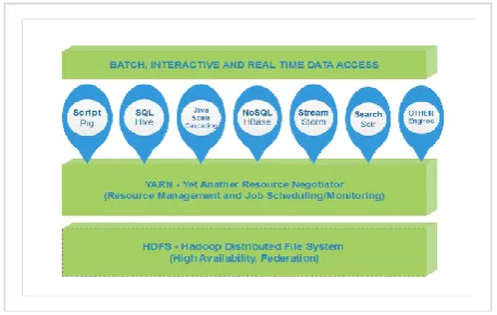
The 1st software (SW) package needed for the cluster is the Hadoop, and in this project the Hadoop 2.7.2 version is used. Hadoop is a big data computing framework that generally refers to the following main components: the Hadoop common utilities, the Hadoop Distributed File System (HDFS) for data storage, the Hadoop Yet Another Resource Negotiator (YARN) for resource management and Job Scheduling/Monitoring and the Hadoop MapReduce which is a YARN-based “Figure 5”. Prerequisite for the Hadoop (SW) to work properly is to choose the proper Java version based on the Hadoop version. As a result, the 2nd software (SW) package we need is Java which is needed to be installed in all the RPi 2 nodes. Hadoop 2.7 version and later require at least Java 7. In this project the oracle-java8-jdk is installed “Figure 3”.

Figure 3: Hadoop and Java version in Hadoop Cluster.

There is another SW package needed to build Hadoop which is the protobuf 2.5.0 libraries. In order to compile the Hadoop binaries, there is a need to apply the HADOOP-9320 patch. Next it’s absolutely necessary to install a whole bunch of

build tools and libraries so as to see the Hadoop, up and running “Figure 4”.

Figure 4: Critical Bunch of build libraries needed for Hadoop setup.

2.3

Hadoop Cluster Architecture

The Apache Hadoop software is based on Java and provides a scalable and fault-tolerant framework for distributed storage and processing of Big Data across many parallel nodes in a cluster. The Apache Hadoop library is designed to scale up from single to thousands nodes, involving hundreds or thousands of terabytes of data, and the library itself is designed to detect and handle failures at the application layer. Hadoop has become the de facto industry framework for Big Data processing because of its innate benefits [5].

Apache Hadoop is composed of two core components, Hadoop Distributed File System (HDFS) and the Hadoop MapReduce which is a YARN-based. The other software or components such as, Hive, HCatalog, Pig, HBase, Sqoop, Mahout, Flume, Oozie, Pegasus and RHadoop are different components that sit on and around Hadoop “Figure 5”.

Figure 5: Hadoop 2.x High Level Architecture.

2.3.1

Hadoop Distributed File System (HDFS)

The Hadoop Distributed File System (HDFS) is based on the Google File System (GFS) and written entirely in Java [6]. Google provided only a white paper with no implementation, but a significant part of the GFS architecture has been applied in its implementation in the form of HDFS.

HDFS is a highly scalable, distributed, load-balanced, portable and fault-tolerant - there is a built-in redundancy at the software level – storage component of Hadoop. In other words, provides high throughput access to application data and is suitable for applications that have large data sets, whereas is designed to run on commodity hardware.

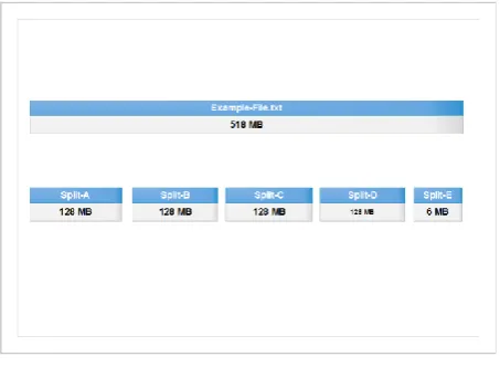
which the master is named Namenode and the slaves are named Datanodes “Figure 6” implementing a distributed file system that provides high-performance access to data. HDFS supports the rapid data transfer between the Datanodes. The master or Namenode manages the file system namespace operations including opening, closing, renaming files and directories and controls access to the files by the client application and multiple Datanodes. The Datanodes manages file storage and storage device attached to it. When HDFS takes the data, internally split them up into one or more blocks – chunks of 128MB by default - and distributes them to different Datanodes in the cluster enabling parallel processing in a high efficient way. The HDFS replicates each piece of data multiple times and distributes the multiple copied data of each block per replication factor to individual Datanodes, placing at least one copy on a different Datanodes than the others. The replication factor is configurable at the cluster level or at file creation. Hence, if the data on Datanodes crash, can be found elsewhere within the cluster performing a highly fault-tolerant operation.

Figure 6: Hadoop HDFS Architecture.

Datanodes are also responsible for serving read and write requests from the HDFS clients and they are performing block creation, deletion and replication when the Namenode instruct them to do. Datanodes store and retrieve blocks when they are instructed to do – by the client application or by the Namenode – and in turn they report back to the Namenode periodically with list of blocks that are stored keeping and informing the Namenode on the current status.

2.3.2

Hadoop MapReduce

MapReduce is generally defined as a programming paradigm to process and generate large set of data [7]. In other words, MapReduce is a software framework – or data processing layer of Hadoop - written in Java and having the ability to split up input data into smaller tasks that can be executed in parallel processes. The output from the so called (map tasks) are then reduced and saved to a file system. In “Figure 7” can be seen the MapReduce flow of a Word Count program where a text file is taken as an input, divided into smaller parts, count each word and outputs a file with a count of all words within a file.

Figure 7: Word Count Flow execution with MapReduce.

A short explanation of the MapReduce Job flow of a Word Count program is depicted below [8], [9].

Split phase. – The so called InputSplits (InputSplits in Hadoop MapReduce is the logical representation of data) are created by logical data division, which serves as the input to a single Mapper Job and the Blocks are created in turn by the physical division of data. One input split can spread across multiple physical blocks of data. The fundamental need of InputSplits is to feed the Mapper with accurate logical data locations so that each Mapper to be able to process complete set of data, spread over more than one blocks. HDFS splits huge files into small ones storing them into the Hadoop file system and those small chunk of spitted data are known as data blocks “Figure 8”. All such things are decided by the Namenode.

Figure 8: InputSplitin Hadoop MapReduce.

InputSplit does not comprise actual data but a reference to the data which is a key-value pair, dependent on the data set and the required output. InputSplit converts the physical representation of a block into logical for the Hadoop mapper, where this block is processed by an individual Mapper. In general, the key-value pair is specified in four places: Map input, Map output, Reduce input and Reduce output. How the input files are split up and read in Hadoop is defined by the InputFormat which is responsible for creating the input splits, dividing them into records. InputSplit in Hadoop is defined by the user according to the size of data. Thus the number of map tasks is equal to the number of InputSplit and the client which runs the job, can calculate the splits for a job, giving this info to the application master to schedule the map tasks that will be processed on the cluster.

generating an intermediate key-value pair and store the intermediate-output on the local disk. Before storing the output for each mapper task, a partitioning of the key of the intermediate-output takes place on the basis of the key and then a sorting is done. The partitioning as a process specifies that all the values of a single key go to the same reducer determining which reducer is responsible for the particular key. The total number of partitioners is equal to the number of reducers. Moreover, the total number of blocks of the input file handles the number of map tasks in a program. As it’s already mentioned, the InputFormat determines in fact the number of maps.

Sort phase. – In this phase, two sub-processes are taking place. The first one is called Shuffling where the intermediate output from mappers are transferred to the reducer and the second is the Sort process which is responsible for merging and sorting of map outputs. The two processes in Hadoop occur at the same time by the MapReduce framework. During the sort phase, all the intermediate key-value pairs generated in mapper in MapReduce are sorted by key, assisting the reducer to distinguish the new reduce tasks when they started.

Reduce phase. – Hadoop Reducer takes as an input a set of an intermediate key-value pair, produced by the mapper aggregated them and then generates the outputs which is the final one and is stored in HDFS. Reducers run in parallel since they are independent of one another.

2.3.3

Yet Another Resource Negotiator (YARN)

YARN is the resource management layer and task scheduling to be executed in different nodes, allocating system resources to the various applications running in a Hadoop cluster. YARN as a cluster resource management layer support different data processing engines, such as graph processing, interactive processing, batch processing and others stored in Hadoop Distributed File System (HDFS). YARN enhances a Hadoop cluster with significant features such as Multi-tenancy where the Capacity Scheduler enables the cluster to be run as multi-tenant systems. In the multi-tenancy architecture, a single instance of a software application serves multiple customers where each customer is named tenant. This ability allows multiple access engines to use Hadoop as a common standard, for interactive, real time and concurrently access the same dataset. The multi-tenancy architecture has a broaden significance in cloud computing because for instance in a Software-as-a-Service (SaaS) provider, we can run one instance of its application on one database instance providing web access to multiple customers. In a Hadoop cluster architecture YARN sits between HDFS and the processing engines which are used to run applications “Figure 9” [10].

Figure 9: Hadoop Cluster resource management – YARN.

2.4

Design and Setup

2.4.1

Design

Hadoop has a Master-Slave architecture for data storage and distributed data processing using MapReduce and Hadoop Distributed File System (HDFS) methods “Figure 10” [11].

Figure 10: Master-Slave architecture in Hadoop.

Master is the node in the cluster which allows to conduct parallel processing of data using Hadoop MapReduce and is named Namenode. Slave is the node which assist to manage the state of an HDFS node, allows to store data to conduct complex calculations and is named Datanode. The JobTracker is an essential Daemon for MapReduce execution, receives the requests for MapReduce execution from the client, determines the data location, and finds the best TaskTracker nodes to execute the tasks, monitoring and controlling the overall status of the job back to clients. The TaskTracker runs on Datanodes which administers the Mapper and Reducer tasks and being in constant communication with the JobTracker signaling the progress of the executed tasks [12], [13], and [14].

The Hadoop cluster is composed of 15 Raspberry Pi’s connected to the 16-Port 10/100 Mbps Ethernet switch. One out of the 15 RPi’s is the master node called Namenode which is the head of the cluster and the rest 14 are the slaves called Datanodes or workers. Each node has a static IP address and the configuration is in such a way where the master can only communicate to every node with secure shell “Figure 11”.

2.4.2

Setup

The fundamental steps of building the cluster, comprises initially a task to set up the network connectivity where the hosts of the cluster must be assigned properly. A dedicated Hadoop user “hduser” and group accounts for the Hadoop environment must be created so as to separate the Hadoop installation from other services. The Rivest-Shamir-Adleman (RSA) key pair to allow “hduser” to access the slave machines seamlessly with empty passphrase is necessary to create in the master node. Secure Shell (SSH) keys replication to all the cluster nodes is necessary so that all the Raspberry Pi’s (RPi’s) to be able to communicate each other without prompting for passwords. Java version "1.8.0_65" must be installed to support Hadoop 2.7.2 version. Then the Hadoop installation and configuration will follow creating the HDFS directories. It’s wise to check and verify the correct Hadoop installation and native libraries using the command “hadoop checknative –a”. The environment variables to be added correctly are very critical, paying attention in the right paths where the Java and Hadoop installation are located.

There are several XML files that must be modified according to our architecture where these modifications needs to be applied in the Namenode and in all the Datanodes. The needed XML files are mentioned briefly below:

Update core-site.xml. – The core-site.xml informs Hadoop daemon where the Namenode runs in the cluster.

Update hdfs-site.xml. – The hdfs-site.xml comprises the configuration setting for HDFS daemons; the Namenode, the secondary Namenode if the cluster architecture is designed so, and the Datanode.

Update yarn-site.xml. – YARN by default tracks Central Processor Unit (CPU) and memory of all nodes, applications, queues and as a resource manager loads its resource definition from the XML configuration files.

Update mapred-site.xml. – The mapred-site.xml comprises the configuration setting for MapReduce daemons; the job tracker and the task-trackers.

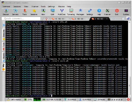
The last step is to format the Namenode and start the services. The right path is in “$HADOOP_HOME/bin/” and the execution command is the “./hdfs namenode –format”. In the Namenode go to “$HADOOP_HOME/sbin/” and execute the commands “./start-yarn.sh” and “./start-dfs.sh” “Figure 12”.

Figure 12: Start Services in Hadoop cluster.

Following starting the services in Hadoop cluster we check with the (Java Virtual Machine Process Status Tool) JPS

command all the Hadoop daemons running on it such as the NameNode, DataNode, ResourceManager, NodeManager etc “Figure 13”.

Figure 13: Hadoop daemons in Namenode and Datanode.

The final verification of the Hadoop cluster that everything is running properly can be done by opening the browser or alternatively the Java processes in the nodes can be checked or to run the HDFS report command “hdfs dfsadmin –report”, “Figure 14”, “Figure 15”.

Figure 14: Namenode overview inHadoop cluster.

3.

PERFORMANCE EVALUATION

3.1

Hadoop HDFS Benchmark

3.1.1

TestDFSIO

The TestDFSIO benchmark is a read and write test for Hadoop Distributed File System (HDFS). That is to say, it will write and read a number of files to and from HDFS and is designed in such a way that it will use one map task per file. The file size and the number of files are specified by the command-line arguments. The TestDFSIO benchmark is part of the “hadoop-mapreduce-client-jobclient.jar”.

The command used for running the write test for instance of 12 files of 1GB each is the following: “hadoop jar /opt/hadoop/share/hadoop/mapreduce/hadoopmapreduceclientjobclient2.7.2.jar TestDFSIO write nrFiles 12 -fileSize 1GB -resFile /tmp/$USER-dfsio-12f-1GBwrite.txt” with the respective results “Figure 16”. Once the preceding command is initiated, a map reduce job will write 12 files to HDFS that are 1 GB in size. These test create data in HDFS under the “/benchmarks/TestDFSIO” directory.

Figure 16: Benchmark of HDFS: Result of write test.

The command used for running the read test for instance of 12 files of 1GB each is the following: “hadoop jar /opt/hadoop/share/hadoop/mapreduce/hadoopmapreduceclientjobclient2.7.2.jar TestDFSIO read nrFiles 12 -fileSize 1GB -resFile /tmp/$ USER-dfsio-12f-1GBread.txt” with the respective results “Figure 17”.

Figure 17: Benchmark of HDFS: Results of read test.

After each test completion it’s needed to clean up the test results, otherwise available storage space will be consumed by the benchmark output file. The command used to clean up test results after completion is the following: “hadoop jar /opt/hadoop/share/hadoop/mapreduce/hadoop-mapreduce-client-jobclient-2.7.2.jar TestDFSIO –clean” “Figure 18.

Figure 18: Clean up test results after completion.

TestDFSIO is designed in such a way that it will use 1 map task per file, namely, it’s a 1:1 mapping from files to map tasks. Splits are defined so that each map gets only one filename, which it creates (-write) or reads (-read). The TestDFSIO benchmark is a read and write stress testing for HDFS, where we discover performance bottleneck in our network, shake out the hardware and give a first impression of how fast our cluster is in terms of I/O. The most notable metrics in TestDFSIO are the Throughput (mb/sec) and the Average IO rate (mb/sec) where both metrics are based on the file size written or read by the individual map, compared with the elapsed time to do it.

Throughput (mb/sec) for a TestDFSIO using (N) map tasks is defined as follows:

(1)

The index denotes the individual map tasks.

The Average IO rate (mb/sec) is defined as follows:

(2)

3.2

Results

3.2.1

TestDFSIO

Table 1. Write Speed Test of Several Files Numb er of Files Total MBytes process ed Throu ghput (mb/se c) Avera ge IO rate (mb/s ec) IO rate standar d deviati on Test exec. time(s ec) 1

1000 1.1670 02

1.167

002 0.00018 2

889.6 83

2

2000 0.9945 66 0.996 609 0.04511 7 2072. 446 3

3000 0.9639 47 0.981 378 0.12575 6 2753. 687 4

4000 1.0609 73 1.075 586 0.11949 1 3200. 846 5

5000 1.0831 82 1.099 735 0.13113 4 4744. 475 6

6000 1.1767 74 1.192 759 0.13712 1 5239. 95 7

7000 1.0801 24 1.113 796 0.18754 8 6661. 712 8

8000 1.2026 52 1.466 353 0.88503 1 6829. 868 9

9000 1.2914 16 1.848 100 1.41464 5 7156. 598 10

10000 1.4058 30 2.058 063 1.45051 9 7303. 195 11

11000 1.4191 48 2.230 232 1.62825 1 7956. 805 12

12000 1.3935 38 2.152 734 1.38241 7 8844. 385

Table 2. Read Speed Test of Several Files

Numb er of Files Total MBytes process ed Throu ghput (mb/se c) Avera ge IO rate (mb/s ec) IO rate standar d deviati on Test exec. time(s ec)

1 ₁₀₀₀ 4.6509

09 4.650 908 0.00212 6 231.8 71 2

2000 4.6914 90 4.691 844 0.04070 8 449.1 42 3

3000 4.7751 83 4.775 540 0.04134 5 657.1 11 4

4000 4.7313 60 4.731 854 0.04803 3 879.8 29 5

5000 4.7598 81 4.760 251 0.04195 3 1090. 584 6

6000 4.7580 06 4.758 788 0.06070 8 1307. 109 7

7000 4.7539 52 4.754 276 0.03907 2 1526. 137 8

8000 4.7150 26 4.715 320 0.03732 6 1757. 054 9

9000 4.7441 30 4.745 264 0.07386 7 1962. 655 10

10000 4.7451 45 4.745 468 0.03930 2 2180. 204 11

11000 4.7796 86 4.780 229 0.05112 5 2377. 444 12

12000 4.7490 13 4.749 453 0.04575 4 2611. 314

A practical example to understand how the Throughput, Average IO rate, Standard Deviation is calculated, is to collect the raw MapReduce results for write and read speed testing by giving the following commands for the writing test (hdfs dfs –cat /benchmarks/TestDFSIO/io_write/part*) and

reading test (hdfs dfs –cat

/benchmarks/TestDFSIO/io_read/part*) respectively “Figure 19”. The following formulas are used to calculate Throughput, Average IO rate, Standard Deviation. [14].

Figure 19: Raw MapReduce result for Write and Read Speed Testing.

Write test Results. – We calculate the Throughput, Average IO rate, Standard Deviation for 5 files 1GB each as depicted in the “Table 1”.

(5)

× = 1.0997354 ×1.0997354= 0.1311344726

The same methodology is used to calculate the read test for 5 files 1GB each, and it’s applied to every experimental result

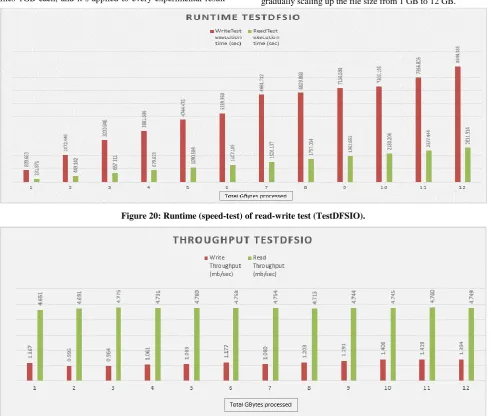
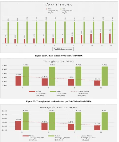
for write and read testing “Table 1”, “Table 2”.

The TestDFSIO read-write test for assessing Hadoop performance was performed by running 1 to 12 files each of size 1GB. In the “Figure 20” we can see the statistics of the read-write TestDFSIO runtime performance, in “Figure 21” we see the throughput TestDFSIO and in “Figure 22” we see the I/O rate TestDFSIO performance based on metrics stated in “Table 1”, “Table 2”. The experimentation started by gradually scaling up the file size from 1 GB to 12 GB.

Figure 20: Runtime (speed-test) of read-write test (TestDFSIO).

Figure 22: I/O Rate of read-write test (TestDFSIO).

Figure 23: Throughput of read-write test per DataNodes (TestDFSIO).

Figure 24: I/O Rate of read-write test per DataNodes (TestDFSIO)

In Hadoop, the tasks are divided among different blocks and the processing is taking place in parallel and independent to each other. With the TestDFSIO read-write testing in fact we examine how efficiently HDFS is able to write and read big files.

It was measured that the read runtime operation is approximately 3.5-4.5 times faster compared to write runtime operation, most likely because the Hard Disk Drive (HDD) in

throughput during reading operation is more by 3.5 to 5 times than the throughput during writing operation. As the number of files is increased, the throughput of the write operation stays approximately the same between (1-7) GB files whereas between (8-12) GB files the throughput starts to increase. In case of read operation the throughput stays approximately the say as the number of files is increased “Table 1”, “Table 2”, “Figure 21”.

The I/O rate is actually the speed where the data transfer takes place between the hard drive, the network and the Random Access Memory (RAM).Concerning I/O rate, as the number of files is increased, the I/O rate of the write operation stays approximately the same between (1-7) GB files whereas between (8 -12) GB, the I/O rate starts to increase “Table 1”, “Table 2”, and “Figure 22”.

Table 3. Write Speed Test to Multiple Nodes

Numbe r of Datano des Total MBytes process ed Throu ghput (mb/se c) Avera ge IO rate (mb/s ec) IO rate standar d deviati on Test exec. time(s ec)

3 ₅₀₀₀ 2.3633

09 2.390 478 0.25311 5 2182. 55 6

5000 1.8038 47 1.828 905 0.20844 8 2860. 783 9

5000 1.6364 90 1.648 843 0.14271 5 3146. 882 12

5000 1.2411 64 1.255 608 0.13355 4 4141. 714

Table 4. Read Speed to Multiple Nodes

Numbe r of Datano des Total MBytes process ed Throu ghput (mb/se c) Avera ge IO rate (mb/s ec) IO rate standar d deviati on Test exec. time(s ec)

3 ₅₀₀₀ 4.7118

97 4.711 999 0.02187 0 1103. 003 6

5000 4.7024 98 4.703 307 0.06175 8 1104. 757 9

5000 4.7115 24 4.713 297 0.09134 3 1102. 966 12

5000 4.7069 72 4.707 448 0.04750 6 1105. 616

Another research interest is to see how the “throughput” and the “average I/O rate” is changing when we increase the “Datanodes” “Table 3”and “Table 4”. Two definite factors that affects the distributed HDFS I/O performance are the block size and the number of Datanodes. The blocks are the units for reading and writing in HDFS. The smaller the block size, the greater the block seek time. In this case the block size considered as the optimal of 128 MB which is the default value. Regarding the number of DataNodes, if the number of

nodes is increased, a sufficient performance improvement is expected due to the increase degree of the distributed data which are processed in parallel. “Figure 23” and “Figure 24” shows the variation of the distributed I/O performance as the number of the DataNodes increases. Instead of the expected results, the throughput” and the “average I/O rate” is linearly decreased when we increase the DataNodes from 3 to 12 “Table 3”, “Table 4”, “Figure 23” and “Figure 24” regarding the writing performance. Compared to read performance the “throughput” and the “average I/O rate” remains constantly the same as the DataNodes increased. The explanation could be that, when the mapping process is completed the resulting blocks are stored in the HDD and then are transferred and received between the DataNodes shuffling through the network. The reading operation does not concern writing in the HDD. On the other hand, in the experiment, all DataNodes are installed in a single Ethernet switch of 100Mbps. It make sense that the bandwidth limitation of the network causes the performance degradation due to overhead of communication between Namenode and DataNodes.

4.

CONCLUSION

In this project, the performance of a Hadoop cluster using commodity low cost HW implemented and analyzed, with the tiny Raspberry Pi 2 platform. The most common benchmarking and testing tools that are included in the Apache Hadoop distribution, are the TestDFSIO, TeraSort, NNBench and MRbench tools. In this project the TestDFSIO used as the most widely reported of these benchmarks. After performing the TestDFSIO benchmark, the following observations can be stated: (a) The HDFS reading operation performance of files is much faster compared to writing operation performance; (b) due to parallel processing the HDFS has good throughput performance; (c) when the DataNodes are increased, the “throughput” and “average I/O rate” performance degradation is observed, concerning the writing operation; (d) the network bandwidth bottleneck seems to be a major factor influencing the whole Hadoop performance;

5.

FUTURE WORK

Since the mVAS dept. is dealing with design, testing and deployment Value Added Services (VAS), and lately started to deal with services in cloud environment there was a huge interest by me to research the Hadoop clustering topic. The first attempt was to design, deploy and stress test an affordable High Performance Hadoop cluster using Raspberry’s Pi 2 so that to gain knowledge and experiment the behavior and performance of a Hadoop cluster with stress testing the MapReduce and HDFS performance. The next step is to combine Hadoop with R programming to investigate the statistical computations and data analysis of massive amounts of data under the scope of Big Data Analytics and distributed machine learning topic.

6.

ACKNOWLEDGMENTS

7.

REFERENCES

[1] Hadoop. [Online]. Available:

https://www.sas.com/el_gr/insights/big-data/hadoop.html

[2] Raspberry Pi 2 Model B. [Online]. Available: https://www.raspberrypi.org/products/raspberry-pi-2-model-b/

[3] Dimitrios Papakyriakou, Dimitra Kottou, and Ioannis Kostouros. Benchmarking Raspberry Pi 2 Beowulf Cluster. International Journal of Computer Applications 179(32):21-27, April 2018. doi: 10.5120/ijca2018916728.

[4] Raspberry Pi 2 Model B. Operating System. [Online]. Available: https://www.raspberrypi.org/downloads/

[5] Apache Hadoop. [Online]. Available: https://hadoop.apache.org/

[6] Sanjay Ghemawat, Howard Gobioff, and Shun-TakLeung. The Google File System, ACM Symposium on Operating Systems Principles, Lake George, NY, pp. 29 – 43, October 2003.

[7] Dean Jeffery, and Sanjay Ghemawat. MapReduce: Simplified Data Processing on Large Clusters. Google Research Publication San Francisco, CA (2004): pp.

137-150 [Online]. Available:

https://static.googleusercontent.com/media/research.goog le.com/en//archive/mapreduce-osdi04.pdf.

[8] Hadoop MapReduce Job Execution flow Chart. [Online]. Available: https://techvidvan.com/tutorials/mapreduce-job-execution-flow/

[9] Srinath Perera and Thilina Gunarathne. Hadoop MapReduce Cookbook. Packt Publishing Ltd, February 2013.

[10] Apache Hadoop YARN. [Online]. Available:

https://hadoop.apache.org/docs/current/hadoop-yarn/hadoop-yarn-site/YARN.html

[11] HDFS Architecture Guide. [Online]. Available: https://hadoop.apache.org/docs/r1.2.1/hdfs_design.html

[12] Hadoop, Architecture, Ecosystem, Components. [Online]. Available: https://www.guru99.com/learn-hadoop-in-10-minutes.html

[13] Tom White. Hadoop: The definitive Guide. O’REILLY, June 2009.