Performance Analysis of a Non-identical Unit System
with Priority and Weibull Repair and Failure Laws
Kuntal Devi
Research Scholar Department of Maths. & Stats.
Manipal University Jaipur Jaipur-303007
Ashish Kumar
Assistant Professor Department of Maths. & Stats.
Manipal University Jaipur Jaipur-303007
Monika Saini
Assistant Professor Department of Maths. & Stats.
Manipal University Jaipur Jaipur-303007
ABSTRACT
The objective of the present paper is to analyze the performance of a two non-identical unit system by considering Weibull distributed random variables. The concept of priority to preventive maintenance of original unit over repair of duplicate unit is also used. A single repairman is available for doing all repair activities. Preventive maintenance of the unit after a pre-specific time to enhance the performance and efficiency of the system conduct by repairman. Recurrence relations for various measures of system effectiveness are derived by using semi-Markov process and regenerative point technique. The system is observed at numerical results for MTSF, steady state availability and profit function has derived for particular case.
Keywords
Non-identical Units; Weibull Failure and Repair Laws; Preventive Maintenance; Priority and Maximum Operation Time
1.
INTRODUCTION
Many researchers like, Cao and Wu [2], Agnihotri and Satsangi [1], Chandrasekhar et al. [3], and Chhillar et al.[4] discussed two-unit cold standby systems under different set of assumptions such as repair, replacement, inspection, etc. Wu and Wu [8] developed stochastic model for standby systems using concept of preventive maintenance after maximum operation time. Zhang and Wang [9] carried out availability analysis of cold standby system with constant failure rate. Some researchers, Osaki and Asakura [7], Gupta et al.[5] and Kumar and Saini [6] suggested some reliability models for cold standby redundant systems and single-unit systems in which all random variables are arbitrary distributed like Weibull distribution.
From the literature highlighted above, we find that a lot of research work is carried out for cold standby unit systems of identical units under the concepts of preventive maintenance and arbitrary distributions. But, the analysis of non-identical unit cold standby systems are not yet discussed by researchers
under arbitrary distributions. For this, here an effort has been made to analyse the performance of a non-identical unit system having one original and one duplicate unit. A reliability model is developed by using concepts of preventive maintenance, repair, replacement and recurrence relations are derived with the help of regenerative point technique and semi-Markov processes for various reliability measures. A single repair facility has been provided to do repair and maintenance activities of original and duplicate unit. After a pre-specific time unit undergoes for preventive maintenance. Random variables are statistically independent and Weibulldistributed. The probability /cumulative density functions of direct transition time from regenerative state i to a regenerative state j or to a failed state j visiting state k, r once in (0, t] have been denoted by qij.kr (t)/Qij.kr(t). The pdf of
failure times of the original and duplicate unit are denoted by 1
( )
exp(
)
f t
t
t
and 12
( )
exp(
)
f t
h t
ht
respectively. Theprobability density function of maximum operation time of original and duplicate unit is denoted by
1
( )
exp(
)
g t
t
t
. The preventivemaintenance rate of the original and duplicate units is denoted by the probability density function
1
1
( )
exp(
)
g t
t
t
. The random variables corresponding to repair rate of the original and duplicate units have the probability density function1
1
( )
exp(
)
f t
k t
kt
and 13
( )
exp(
)
f t
l t
lt
respectively with0
Nomenclature
O Operative unit
DCs Duplicate cold standby unit Do Duplicative unit is operative
~ / * Symbol for Laplace -Steiltjes Transform (LST) / Laplace Transfor(LT) Ⓢ/
Symbol for Laplace-Stieltjes convolution/Laplace convolution Fur/FUR Denotes the failed original unit under repair/continuously under repair DFur/DFUR Denotes the failed duplicate unit under repair/continuously under repairDPm/DPM Denotes that duplicate unit under preventive maintenance/ continuously under preventive maintenance
Pm/PM Denotes that original unit under preventive maintenance/ continuously under preventive maintenance WPm/WPM Denotes that original unit waiting for preventive maintenance/ continuously waiting for preventive
maintenance
DWPm/DWPM Denotes that duplicate unit waiting for preventive maintenance/ continuously waiting for preventive maintenance
Fwr/FWR Original unit after failure waiting for repair/continuously waiting for repair DFwr / DFWR Duplicate unit after failure waiting for repair/continuously waiting for repair MTSF Mean Time to System Failure
2. MODEL DESCRIPTION
In this section, a stochastic model has been developed for two non-identical unit’s systems using the concept of priority and arbitrary distributions. The system may be any of the following states describes as follows:
0 1 2 3 4
5 6 7 8
9 10 11 12
( , ), ( , ), ( , ), ( , ), ( , ),
( , ), ( , ), ( , ), ( , ),
( , ), ( , ), ( , ), ( , ),
S O Dcs S Pm Do S Fur Do S O DFur S O DPm
S Fwr DPM S FUR DFwr S FUR DPwm S WPm DPM
S PM DPwm S PM DFwr S Fwr DFUR S Pm DFwr
Out of these states
S
0S
1S
2S
3 andS
4are the operative and regenerative states while all other are non-regenerative and failed states.3.
TRANSITION PROBABILITIES AND
MEAN SOJOURN TIMES
Simple probabilistic considerations yield the following expressions for the non-zero elements
ij ij ij
p = Q (
)= q (t)dt
As (1)p01=
, p02=
, p10 =h
, p1.10 =h
h
=p13.10, p19=h
=p14.9,p20 =
k
k
h
, p26 =h
h k
=p23.6, p27 =h k
= p24.7, p30 =l
l
, p40 =
,p3.12 =
l
= p33.12, p3.11 =l
= p32.11, p45=
= p42.5, p48=
= p44.8,It can be easily verified that sum of all transition probabilities from each state is one.
4.
PERFORMANCE MEASURES:
4.1 Reliability and Mean Time to System
Failure (MTSF)
Let
φ t
i
be the cdf of first passage time from the regenerative state i to a failed state. Regarding the failed state as absorbing state, we have the following recursive relations for
iφ t
:
i i, j j i,k
j k
φ t =
Q
t ®φ t + Q
t
(3)Where j is an un-failed regenerative state to which the given regenerative state i can transit and k is a failed state to which the state i can transit directly. Taking LST of above relation (3) and solving for
0( )
s
.The mean time to system failure(MTSF) is given by MTSF = 0 0
1
lim
sφ (s)
s
4.2 Steady State Availability
Let Ai(t) be the probability that the system is in up-state at
instant 't' given that the system entered regenerative state i at t = 0. The recursive relations for Ai (t) are given as
( )
,n
i i i j j
j
A t
M t
q
t
A t
(4)Where j is any successive regenerative state to which the regenerative state i can transit through n transitions. Taking
LT of above relations (4) and solving for
* 0
( )
A s
. The steadystate availability is given by
*
0 0
0
( )
lim
( )
s
A
sA s
(5)4.3 Busy Period Analysis for Server
Let
B
iR(
t
)
andB
iPm(t)
be the probability that the server is busy in repairing and preventive maintenance of the unit at an instant ‘t’ given that the system entered state i at t = 0. The recursive relations forB
iR(
t
)
are as follows:
( )
,n
R R
i i i j j
j
B
t
W t
q
t
B
t
, ipm
i
i j( ),n
pmj
jB
t
W t
q
t
B
t
(6)Where j is any successive regenerative state to which the regenerative state i can transit through n transitions. By taking LT of (6) and solving for
B
0*R( )
s and B
0*Pm( )
s
. The busy period of the server due to repair and PM is given by* *
0 0
0 0
lim
,
lim
R R Pm Pm
0 0
s s
B =
sB (s) B
=
sB
(s)
4.4 Expected Number of Repairs, PM and
Visits by Server
Let
E (t)
iR ,E
iPm(t)
and Ni(t) be the expected number ofrepairs PM and visits by the server in (0, t] given that the system entered the regenerative state i at t = 0. The recursive relations for these are given as
( )
, n
R R
i i j j j
j
E
t
Q
t
E
t
, iPm
i j( ),n
j Pmj
jE
t
Q
t
E
t
( )
, n
i i j j j
j
N
t
Q
t
N
t
(7)Where j is any regenerative state to which the given regenerative state i transits and
δj
=1, if j is the regenerative state where the server does job afresh, otherwiseδj
= 0.Taking LST of relations (7) and solving for 0 R
E (s)
. The expected numbers of repairs per unit time are given by0 0
( )
lim
0( )
R R
s
E
s E
s
, 0 00
( )
lim
( )
Pm Pms
E
s E
s
and 0 0
0
( )
lim
( )
sN
sN s
(8)0 0 1 0 2 0 3 0 4 0 5 0
Pm R Pm R
P
K A
K B
K B
K E
K E
K N
(9)
K0 = Revenue per unit up-time of the system
Ki = Cost per unit time for which server is busy due various
5.
NUMERICAL RESULTS
Table 1: MTSF vs. Failure Rate (β) for shape parameter η=0.5
[image:4.595.49.504.101.250.2]β α=2,η=0.5, γ=5,k=1.5, h=0.009, l=1.4 α=2.4,η=0.5, γ=5,k=1.5, h=0.009, l=1.4 α=2,η=0.5, γ=7,k=1.5, h=0.009, l=1.4 α=2,η=0.5, γ=5,k=1.5, h=0.01, l=1.4 α=2,η=0.5, γ=5,k=1.7, h=0.009, l=1.4 α=2,η=0.5, γ=5,k=1.5, h=0.009, l=2 0.01 0.02 0.03 0.04 0.05 0.06 0.07 0.08 0.09 0.1 4.9918 4.7950 4.6123 4.4423 4.2836 4.1351 3.9960 3.8654 3.7426 3.6268 2.1095 2.0642 2.0207 1.9788 1.9385 1.8998 1.8624 1.8264 1.7916 1.7581 11.7910 10.7622 9.8940 9.1515 8.5094 7.9487 7.4548 7.0165 6.6251 6.2733 4.9821 4.7861 4.6040 4.4345 4.2763 4.1283 3.9896 3.8594 3.7369 3.6214 6.6949 6.3613 6.0577 5.7803 5.5260 5.2919 5.0758 4.8757 4.6898 4.5169 4.9918 4.7950 4.6123 4.4423 4.2836 4.1351 3.9960 3.8654 3.7426 3.6268
Table 2: MTSF vs. Failure Rate (β) for shape parameter η=1.0
[image:4.595.52.500.468.614.2]β α=2,η=1,γ=5,k =1.5,h=0.009, l=1.4 α=2.4,η=1,γ=5,k =1.5, h=0.009, l=1.4 α=2,η=1, γ=7,k=1.5, h=0.009, l=1.4 α=2,η=1, γ=5,k=1.5, h=0.01, l=1.4 α=2,η=1, γ=5,k=1.7, h=0.009, l=1.4 α=2,η=1, γ=5,k=1.5, h=0.009, l=2 0.01 0.02 0.03 0.04 0.05 0.06 0.07 0.08 0.09 0.1 5.9647 5.7599 5.5696 5.3921 5.2264 5.0712 4.9255 4.7886 4.6596 4.5379 3.0460 2.9933 2.9426 2.8937 2.8466 2.8012 2.7573 2.7150 2.6741 2.6346 13.8080 12.6725 11.7138 10.8934 10.1835 9.5632 9.0165 8.5310 8.0970 7.7067 5.9531 5.7491 5.5594 5.3826 5.2174 5.0627 4.9176 4.7811 4.6525 4.5312 8.0001 7.6420 7.3158 7.0175 6.7437 6.4914 6.2583 6.0422 5.8414 5.6542 5.9647 5.7599 5.5696 5.3921 5.2264 5.0712 4.9255 4.7886 4.6596 4.5379
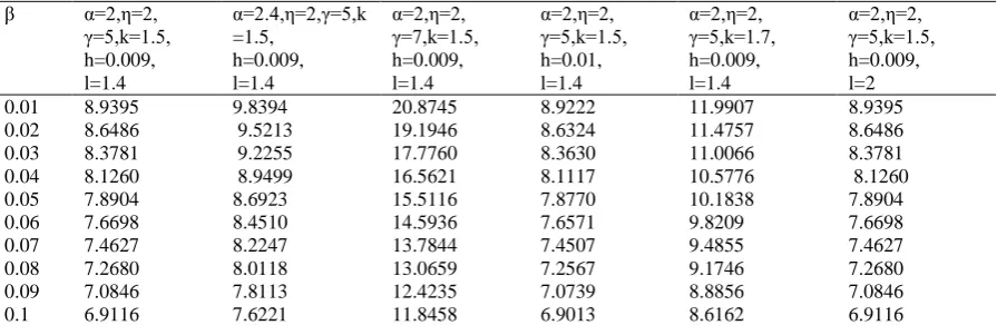
Table 3: MTSF vs. Failure Rate (β) for shape parameter η=2.0
[image:4.595.51.501.651.768.2]β α=2,η=2, γ=5,k=1.5, h=0.009, l=1.4 α=2.4,η=2,γ=5,k =1.5, h=0.009, l=1.4 α=2,η=2, γ=7,k=1.5, h=0.009, l=1.4 α=2,η=2, γ=5,k=1.5, h=0.01, l=1.4 α=2,η=2, γ=5,k=1.7, h=0.009, l=1.4 α=2,η=2, γ=5,k=1.5, h=0.009, l=2 0.01 0.02 0.03 0.04 0.05 0.06 0.07 0.08 0.09 0.1 8.9395 8.6486 8.3781 8.1260 7.8904 7.6698 7.4627 7.2680 7.0846 6.9116 9.8394 9.5213 9.2255 8.9499 8.6923 8.4510 8.2247 8.0118 7.8113 7.6221 20.8745 19.1946 17.7760 16.5621 15.5116 14.5936 13.7844 13.0659 12.4235 11.8458 8.9222 8.6324 8.3630 8.1117 7.8770 7.6571 7.4507 7.2567 7.0739 6.9013 11.9907 11.4757 11.0066 10.5776 10.1838 9.8209 9.4855 9.1746 8.8856 8.6162 8.9395 8.6486 8.3781 8.1260 7.8904 7.6698 7.4627 7.2680 7.0846 6.9116
Table 4: Availability vs. Failure Rate (β) for shape parameter η=0.5
0.08 0.09 0.1 0.9067 0.9020 0.8973 0.8664 0.8608 0.8553 0.9387 0.9338 0.9290 0.9067 0.9019 0.8972 0.9159 0.9122 0.9085 0.9069 0.9021 0.8974
Table 5: Availability vs. Failure Rate (β) for shape parameter η=1.0
[image:5.595.55.501.323.470.2]β α=2,η=1,γ=5, k=1.5,h=0.00 9, l=1.4 α=2.4,η=1,γ=5,k =1.5, h=0.009, l=1.4 α=2,η=1, γ=7,k=1.5, h=0.009, l=1.4 α=2,η=1, γ=5,k=1.5, h=0.01, l=1.4 α=2,η=1, γ=5,k=1.7, h=0.009, l=1.4 α=2,η=1, γ=5,k=1.5, h=0.009, l=2 0.01 0.02 0.03 0.04 0.05 0.06 0.07 0.08 0.09 0.1 0.8944 0.8919 0.8894 0.8869 0.8845 0.8821 0.8797 0.8773 0.8749 0.8726 0.8623 0.8598 0.8573 0.8549 0.8525 0.8501 0.8477 0.8453 0.8430 0.8407 0.9371 0.9343 0.9315 0.9288 0.9261 0.9234 0.9207 0.9180 0.9154 0.9128 0.8943 0.8918 0.8893 0.8869 0.8844 0.8820 0.8796 0.8772 0.8749 0.8725 0.8948 0.8927 0.8906 0.8885 0.8864 0.8844 0.8823 0.8803 0.8783 0.8763 0.8945 0.8920 0.8895 0.8870 0.8846 0.8822 0.8798 0.8774 0.8750 0.8727
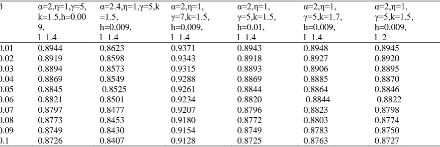
Table 6: Availability vs. Failure Rate (β) for shape parameter η=2.0
[image:5.595.57.500.497.644.2]β α=2,η=2, γ=5,k=1.5, h=0.009, l=1.4 α=2.4,η=2, γ=5,k=1.5, h=0.009, l=1.4 α=2,η=2, γ=7,k=1.5, h=0.009, l=1.4 α=2,η=2, γ=5,k=1.5, h=0.01, l=1.4 α=2,η=2, γ=5,k=1.7, h=0.009, l=1.4 α=2,η=2, γ=5,k=1.5, h=0.009, l=2 0.01 0.02 0.03 0.04 0.05 0.06 0.07 0.08 0.09 0.1 0.8715 0.8700 0.8686 0.8671 0.8657 0.8643 0.8629 0.8615 0.8601 0.8587 0.8452 0.8438 0.8425 0.8411 0.8398 0.8385 0.8372 0.8359 0.8346 0.8333 0.9109 0.9092 0.9076 0.9059 0.9043 0.9026 0.9010 0.8995 0.8979 0.8963 0.8714 0.8700 0.8685 0.8670 0.8656 0.8642 0.8628 0.8614 0.8600 0.8586 0.8717 0.8704 0.8691 0.8678 0.8666 0.8653 0.8641 0.8628 0.8616 0.8604 0.8716 0.8701 0.8687 0.8672 0.8658 0.8644 0.8630 0.8616 0.8602 0.8588
Table 7: Profit vs. Failure Rate (β) for shape parameter η=0.5
[image:5.595.47.500.678.769.2]β α=2,η=0.5, γ=5,k=1.5, h=0.009, l=1.4 α=2.4,η=0.5, γ=5,k=1.5, h=0.009, l=1.4 α=2,η=0.5, γ=7,k=1.5, h=0.009, l=1.4 α=2,η=0.5, γ=5,k=1.5, h=0.01, l=1.4 α=2,η=0.5, γ=5,k=1.7, h=0.009, l=1.4 α=2,η=0.5, γ=5,k=1.5, h=0.009, l=2 0.01 0.02 0.03 0.04 0.05 0.06 0.07 0.08 0.09 0.1 5932.3 5912.0 5891.7 5871.4 5851.2 5831.0 5810.8 5790.6 5770.5 5750.4 6232.2 6203.7 6175.3 6147.1 6119.1 6091.3 6063.6 6036.1 6008.8 5981.6 6156.2 6135.8 6115.5 6095.2 6074.8 6054.5 6.034.2 6014.0 5993.7 5973.5 5932.1 5911.8 5891.5 5.871.2 5850.9 5830.7 5810.5 5790.3 5770.2 5750.1 5940.0 5927.4 5914.7 5901.9 5889.1 5876.3 5863.5 5850.6 5837.7 5824.7 5933.0 5912.8 5892.5 5872.3 5852.2 5832.0 5811.9 5791.8 5771.7 5751.7
Table 8: Profit vs. Failure Rate (β) for shape parameter η=1.0
0.01 0.02 0.03 0.04 0.05 0.06 0.07 0.08 0.09 0.1
5324.7 5312.1 5299.6 5287.2 5275.0 5262.8 5250.7 5238.8 5226.9 5215.1
5326.4 5316.3 5306.2 5296.2 5286.3 5276.5 5266.7 5257.0 5247.4 5237.8
5323.6 5310.9 5298.4 5286.0 5273.7 5261.5 5249.4 5237.4 5225.6 5213.8
5640.6 5626.3 5612.1 5598.1 5584.2 5570.5 5.556.8 5543.3 5530.0 5516.7
5276.8 5263.8 5250.9 5238.1 5225.4 5.212.9 5200.4 5188.0 5175.8 5163.6
[image:6.595.58.500.220.368.2]5323.9 5311.3 5298.8 5286.4 5274.1 5261.9 5249.8 5237.8 5226.0 5214.2
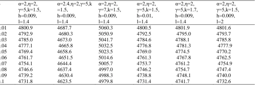
Table 9: Profit vs. Failure Rate (β) for shape parameter η=2.0
β α=2,η=2, γ=5,k=1.5, h=0.009, l=1.4
α=2.4,η=2,γ=5,k =1.5,
h=0.009, l=1.4
α=2,η=2, γ=7,k=1.5, h=0.009, l=1.4
α=2,η=2, γ=5,k=1.5, h=0.01, l=1.4
α=2,η=2, γ=5,k=1.7, h=0.009, l=1.4
α=2,η=2, γ=5,k=1.5, h=0.009, l=2 0.01
0.02 0.03 0.04 0.05 0.06 0.07 0.08 0.09 0.1
4800.9 4792.9 4785.0 4777.1 4769.4 4761.7 4754.1 4746.6 4739.2 4731.8
4687.7 4680.3 4673.0 4665.8 4658.6 4651.5 4644.4 4637.4 4630.4 4623.5
5060.3 5050.9 5041.7 5032.5 5023.5 5014.6 5005.7 4997.0 4988.3 4979.8
4800.5 4792.5 4784.6 4776.8 4769.0 4761.3 4753.7 4746.2 4738.8 4731.4
4801.9 4795.0 4788.1 4781.3 4774.5 4767.8 4761.2 4754.7 4748.1 4741.7
4801.6 4793.7 4785.8 4777.9 4770.2 4762.5 4754.9 4747.4 4740.0 4732.6
6.
CONCLUSION
In the section entitled numerical results, we obtained numerical values of performance measures such as mean time to system failure, availability and profit function for the proposed model with respect to failure rate (λ) for various values of shape parameter η=0.5, 1, 2. For η=1, all random variables behaves as exponential distribution as a particular case of Weibull distribution while for η=2, it becomes Rayleigh. From, tables 1-9, we observe that the availability and profit of the system model decreases while MTSF increases with the increase of shape parameter. These measures shows a steep decline with the increase of failure rate of original and duplicate unit, maximum operation time whereas increase with respect to preventive maintenance of system and repair and replacement of original and duplicate unit. Finally, we conclude that by increasing the repair rate of the original and duplicate unit system can be made more profitable.
7.
REFERENCES
[1] R. R. Agnihotri, S.K.Satsangi, Two Non-identical unit system with priority based repair and inspection, Microelectronic reliability, 36(2), 1996, 279-282. [2] J. Cao, Y. Wu, Reliability analysis of a two-unit cold
standby system with a Replaceable repair facility, Microelectronics Reliability, 29(2), 1989, 145-150. [3] P. Chandrasekhar, R. Natarajan, V. S. S. Yadavalli, A
study on a two unit standby System with Erlangian repair
Time, Asia-Pacific Journal of Operational Research, 21(03), 2004, 271-277.
[4] S. K. Chhillar, A. K. Barak, S. C. Malik, Reliability measures of a cold standby system with priority to repair over corrective maintenance subject to random shocks, International Journal of Statistics & Economics™,13(1), 2014, 79-89.
[5] R. Gupta, P. Kumar, A. Gupta, Cost-benefit analysis of a two dissimilar unit cold standby system with Weibull failure and repair laws, Int. J. Syst. Assur. Eng. Manag., 4(4), 2013, 327–334.
[6] A. Kumar, M. Saini, Cost-benefit analysis of a single-unit system with preventive maintenance and Weibull distribution for failure and repair activities, Journal of Applied Mathematics, Statistics and Informatics, 10(2), 2014, 5-19.
[7] S. Osaki, T. Asakura, A two-unit standby redundant system with repair and preventive maintenance, Journal of Applied Probability, 7, 1970, 641-648.
[8] Q. Wu, S. Wu, Reliability analysis of two-unit cold standby repairable systems under Poisson shocks, Applied Mathematics and computation, 218(1), 2011, 171-182.