Distributed Control of Battery Energy Storage
System in a Microgrid
Jie Ma
Engineering Department, Lancaster University Lancaster, United Kingdom
j.ma6@lancaster. ac.uk
Xiandong Ma
Engineering Department, Lancaster University Lancaster, United Kingdom
Abstract—Due to the high penetration of renewable power system with variable generation profiles, the need for flexible demand and flexible energy storage increases. In this paper, a hierarchical energy dispatch scheme incorporating energy storage system is presented to address the uncontrollability of renewable power generation. Statistical-based forecasting techniques are preformed and compared in order to accurately predict solar radiance and estimate solar power generation. Battery energy storage system (BESS) is often deployed as a flexible power supplier to reduce the peak power, emissions and cost. This paper elaborates a multi-agent system (MAS) based distributed algorithm to investigate an energy dispatch scheme for BESS, based on the renewable energy forecasting results. A 24-hour prescheduled energy dispatch scheme is assigned to individual BESSs based on IEEE 5-bus system and IEEE 14-bus system. Simulation results are shown to demonstrate the feasibility and scalability of the algorithm,
Keywords--hierarchical energy dispatch scheme; BESS; MAS-based distributed algorithm; forecasting techniques
I. INTRODUCTION
The trend of developing low carbon economy and green energy generation in power systems has resulted in the installation of more distributed generation (DG) resources and energy storage systems (ESS). The uncontrollability and intermittency of weather condition poses a great challenge to maintain a stable power supply. In order to overcome this problem, many intelligent computational methods have been employed to predict on-site weather condition and estimate renewable power generation [1], [2][3]. The widely-used weather forecasting techniques can be classified into three mainstreams: numerical prediction, statistical approaches, artificial intelligent algorithms and hybrid models. As presented in [4], [5], authors gave an in-depth review of solar radiance forecasting methods in small-scale area. Subjected to measurement of solar radiance, many researchers investigated the effects of various weather indexes on predicting solar radiance. Conventionally, temperature, humidity and wind speed have been regarded as the highest relevant factors for solar radiance. Temperature, sky information and solar irradiance level were integrated into a hybrid model in reference [6], where its forecasting accuracy outperformed single intelligent algorithm. Reference [7] investigated the extremely weather condition, where aerosol index was used as an optimal indicator to record solar radiance attenuation. In [8], the authors summarised a number of solar forecasting models based on different weather types.
In an autonomous microgrid system, the employment of the BESSs aims to stabilize the system frequency and voltage by regulating the active power and reactive power. Many literatures have studied the control and optimization of BESSs[9][10][11][12]. For example. reference [9] presented a droop control protocol for distributed BESS to regulate grid frequency and reduce the impact of unstable renewable generation. In [13], an adaptive droop control was proposed for balancing the SoC (state of charge) of the distributed BESSs. However, all studies assume that the charging/discharging efficiency is constant for different charging/discharging rate. Furthermore, renewable generation forecasting has not been considered in the existing researches.
In this paper, solar radiance history data, temperature, ultraviolet index and weather type are selected as exogenous variables of the forecasting model while the statistical technology is employed to deal with time-series forecasting problem. A hybrid method combining MAPA (Multiple Aggregation Prediction Algorithm) and PCA (principal components analysis) model is presented to forecast solar radiance, as demonstrated in Section II. Section III introduces a MAS-based energy dispatch scheme to maintain the active power balance along with the BESS charging and discharging efficiency. In Section IV, four case studies are performed to test the feasibility of the algorithm with and without power constraints and to assess its scalability and robustness, followed by the conclusions.
II. RENEWABLE ENERGY FORECASTING
Wind and solar, as the environmentally friendly natural energy, are typically resources for renewable power generators. Due to its uncertainty and uncontrollability, renewable energy brings a great challenge in order to provide a stable power supply for end users. A real-time weather forecasting dataset acquired from the Met office is employed to indirectly predict local solar radiance. Met office is a national weather service in the UK, which updates a set of weather forecasting indexes every 3 hours for next 5 day covering all of weather observation sites. In this paper, development of a hybrid model incorporating statistical approaches is the focus, aiming to predict local solar radiance based on available weather indexes and historical solar radiance data.
selected to predict solar radiance𝑌𝑡. The UV index, temperature and weather type are used as explanatory variables 𝑋𝑖. Considering the updating resolution of weather forecasting data, the solar radiance can be predicted with the frequency of every 3 hours.
𝑌𝑡 = 𝛼0+
∑
8𝑖=1𝛽𝑖𝐷𝑖+∑
3𝑗=1𝛾𝑗𝑋𝑖+∑
𝑘=1,2,8𝛿𝑘𝑌𝑡−𝑘 (1)where 𝛼0 is an estimation of true level. In order to capture the seasonality in a time-series dataset, dummy variable 𝐷𝑖 is introduced to describe 3-hourly seasonality. 𝑌𝑡−1, 𝑌𝑡−2, 𝑌𝑡−8 represent the lag variables (lagged approximately by 3, 6 and 24 hours, respectively) to analyse the effects of historical data on current variable 𝑌𝑡. The 𝛽𝑖, 𝛾𝑗, 𝛿𝑘 are coefficients of different regressors. As an example, Fig 1 shows short-term solar radiance forecasting results with the multiple linear regression model. Clearly, the estimated value follows the observation data, with the mean absolute percentage error (MAPE) and coefficient of determination (R-square) being 69.27 and 0.745 respectively.
Autoregressive integrated moving average (ARIMA) model, as a widely used statistic technique, is used to fit time series data. AR (autoregressive) part explains that the forecast variable is regressed on its own lag values. MA (moving average) term indicates the regression error is a linear combination of error terms whose value occurs at various times in the past. I (integration) part is used to replace the data with data difference between the current value and previous values. The use of each component aims to make the model fit the data as accurately as possible. The model is denoted by ARIMA (𝑝, 𝑑, 𝑞), where the non-negative parameters 𝑝, 𝑑, 𝑞 are the order of AR, I and MA models, respectively. Mathematically, it can be written as
(
1 −∑
𝑝𝑖=1𝜙𝑖𝐿𝑖)(
1 − 𝐿)
𝑑𝑌𝑡=(
1 −∑
𝜃𝑖𝐿𝑖 𝑞𝑖=1
)
𝜀𝑡 (2)where L is the lag operator,𝜙𝑖 and 𝜃𝑖 are parameters of AR and MA of model, respectively, 𝜀𝑡 is error terms. Generally, ARIMA model can be estimated with Box-Jenkins approach, where a range of candidate models can be evaluated by Akaike Information Criterion (AIC), in order
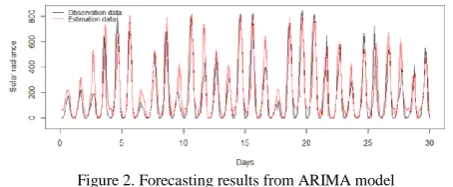
to investigate the optimal order and parameters in the model. Fig 2 shows the forecasting result from ARIMA model, with MAPE and coefficient of determination being 86.67 and 0.78, respectively.
B. MAPAx -PCA hybrid model
Multiple Aggregation Prediction Algorithm (MAPA) proposed by Kourentzes et al. takes advantage of time series transformation by aggregating time series data into different temporal levels [14]. This approach makes its components (trend, level, seasonality) become more or less prominent with the direct effect on forecast model identification and estimation.
MAPA can be implemented in a three-step procedure. In the first step, the original time series data is aggregated into multiple aggregation levels by means of length 𝑘, where the aggregated time series is smoother than original data. High frequency components are progressively attenuated with the increase of the aggregation level, thus filtering the seasonality and outlier components. In contrast, low frequency components (trend and level) are captured and dominant in the forecast model. In second step, forecasting techniques such as exponential smoothing (ETS) model can be fitted at each aggregation level, where the level, trend and seasonality can be extracted, respectively. AIC is used to evaluate each ETS model. The component prediction can be estimated with the law as referenced in [10]. The last step involves the combination of components estimation across different aggregation levels, where two combination schemes were proposed, namely weighted mean and median.
MAPA can be extended to include exogenous variables, which is named as MAPAx. Similarly, exogenous multivariable should be aggregated into different temporal level, respectively, which is denoted by 𝑋𝑗[𝑘]. All of aggregation levels for each variable can be combined into a single effect 𝑋𝑗. The input variables are incorporated into the ETS model and univariable forecasting result is then adjusted with multivariable effect estimation, where the structure of MAPAx algorithm is demonstrated in Fig 3.
However, as 𝑋𝑗 aggregated, the correlation between each explanatory variable is changed and potentially cause the multicollinearity at the higher aggregation level, if there are more than one explanatory variable considered in the model. This problem appears if lag variables are introduced to the model, which can be solved by transforming the variables into associated orthogonal coefficients with principal components analysis (PCA). Mathematically, PCA is performed by an orthogonal linear transformation of the data into a new coordinate system, where the first principle component has the greatest variance of the
[image:2.595.58.287.339.416.2]Identify applicable sponsor/s here. (sponsors)
Figure 1. Forecasting results from the multiple linear regression model
Figure 2. Forecasting results from ARIMA model
Input
Times Series Y [k]
Times Series X[k]
i
Principal Components
Analysis Exponential Smoothing Fit
Additive Translation
l[k] t+h
t[k] t+h
s[k] t+h
d[k] t+h
Y[1] t+h
Univariate
Exogenous
Output Forecasting
[image:2.595.309.537.533.642.2] [image:2.595.58.285.671.764.2]original data and comes to lie on the first coordinate. The succeeding component on the second coordinate has the second greatest variance under the constraint that it is orthogonal to the preceding components. Therefore, the new set of variables 𝑋̂𝑖generated by PCA are no longer
multicollinear and contain no redundant information. Replacing the original variables with the orthogonal principal components can address the multicollinearity problem. To produce the final forecasting for ℎ steps ahead, the algorithm is implemented as below.
The forecasting results can be seen in Fig 4. Compared
with Fig 1 and Fig 2, the MAPE from the MAPA-PCA hybrid model is 65.0355 and its coefficient of determination is 0.803, demonstrating a better fitting performance.
C. Solar radiance and solar power forecasting
Given solar radiance reference value 𝑆𝑟𝑒𝑓= 1000W/ 𝑚2 and temperature reference value 𝑇𝑟𝑒𝑓 = 25℃, the real time power output under arbitrary solar radiances and temperatures can be estimated. Provided a set of reference parameters (short-circuit current 𝐼𝑠𝑐, open circuit voltage 𝑉𝑜𝑐, maximum current 𝐼𝑚 and maximum voltage 𝑉𝑚) under 𝑆𝑟𝑒𝑓 and 𝑇𝑟𝑒𝑓, these parameters under a real situation can be calculated as.
𝐼𝑠𝑐′ = 𝐼𝑠𝑐 𝑆
𝑆𝑟𝑒𝑓(1 + 𝛼∆𝑇) (3a)
Voc′ = Uoc(1 − γΔT)In(1 + 𝛽𝛥𝑆) (3b)
𝐼𝑚′ = 𝐼𝑚 𝑆
𝑆𝑟𝑒𝑓(1 + 𝛼Δ𝑇) (3c)
𝑉𝑚′ = 𝑈𝑚
(
1 + 𝛾∆𝑇)
In(1 + 𝛽𝛥𝑆) (3d)where ∆𝑇 = 𝑇 − 𝑇𝑟𝑒𝑓 and 𝛥𝑆 = 𝑆 𝑆⁄ 𝑟𝑒𝑓− 1. Assume that the shape of output characteristic (IV curve) remains unchanged, the parameters 𝛼, 𝛽 and 𝛾 can be set as 0.0025/℃ , 0.5 and 0.00288/℃ , respectively. The calculated parameters 𝐼𝑚
′
and 𝑈𝑚 ′
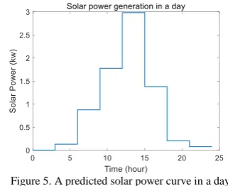
can be used to estimate the maximum power output, if solar PV always operates at the maximum power point. Suppose that there is a PV array with 4 parallel strings and 6 series-connected modules per string installed in a house roof. Taking the solar radiance forecasting in 3rd July as an example, the daily solar power
curve can be calculated as shown in Fig 5. The outcome will be integrated into control strategy to evaluate the robustness of distributed algorithm. More details will be elaborated in case study 2.
III. MAS-BASED DISTRIBUTED ALGORITHM OF BESS
A. Problem formulation
The active power balance problem in an autonomous microgrid system can be represented as
𝑃𝐷=∑𝑃𝐺,𝑖−∑𝑃𝐿,𝑖 (4)
where 𝑃𝐷 is total supply-demand mismatch, 𝑃𝐺,𝑖 and 𝑃𝐿,𝑖 are active power generation and load demand at the 𝑖𝑡ℎ bus, respectively. Due to the intermittency of the renewable power generation, BESS is employed to compensate power imbalance, which is formulated as
𝑃𝐷=∑𝑃𝐵,𝑖 (5)
where 𝑃𝐵,𝑖 is charging/discharging active power of BESS at the 𝑖𝑡ℎ local bus. In order to obtain an optimal charging efficiency, the cost function of BESS can be formulated as quadratic convex function C(𝑃𝐵,𝑖), when BESS operates in the normal power range ( 𝑃𝐵,𝑖𝑚𝑖𝑛< 𝑃𝐵,𝑖< 𝑃𝐵,𝑖𝑚𝑎𝑥 ), as referenced in [15]. The incremental cost 𝜆𝑖 can be defined as:
𝜆𝑖= ∂C(𝑃𝐵,𝑖)
∂𝑃𝐵,𝑖 = 𝑎𝑖− 2𝑏𝑖𝑃𝐵,𝑖 (6)
The solution to eq. (6) is the equal incremental cost criterion introduced by [16], which is equal to
𝜆∗= ∑𝑎𝑖
2𝑏𝑖−𝑃𝐷
∑1
2𝑏𝑖
(7)
The associated optimal charging power of each individual BESS can be calculated as.
𝑃𝐵,𝑖∗ = −𝜆∗+𝑎𝑖
2𝑏𝑖 (8)
MAPAx implementation
1. Given a time series forecast variable 𝑌 = {𝑌𝑡} and exogenous variables 𝑋 = {𝑋𝑖,𝑡} with 𝑡 = 1,2, … , 𝑁, 𝑖 = 1,2, … , 𝑚. N is number of samples whereas as m is the number of exogenous variables. 2. Preprocess multicollinearity for those exogenous variables with PCA to produce a new exogenous variable set 𝑋̂ = {𝑋̂𝑖,𝑡}
3. Temporally aggregating time series into different level 𝑧𝑖[𝑘]=
𝑘−1∑ 𝑧
𝑡 𝑖𝑘
𝑡=1−(𝑖−1)𝑘 , where 𝑧𝑡= {𝑌, 𝑋̂}, 𝑘 = 1,2, … , 𝑇, 𝑑𝑗,𝑡[𝑘]=
𝑐𝑖[𝑘]𝑋̂𝑗 [𝑘]
, where 𝑑𝑗,𝑡 is the effect of the each 𝑋̂𝑗 variable, 𝑐𝑖[𝑘] is the weighting coefficients, T is time period of 𝑌𝑡
4. Fit ETS Model components (level, trend and seasonality) at each aggregation level {𝑙𝑡+ℎ[𝑘], 𝑡𝑟𝑡+ℎ[𝑘], 𝑠𝑡+ℎ[𝑘], 𝑑𝑡+ℎ[𝑘] }
5. Weights combination scheme. 𝑌̂[1]= ∑ 𝛼 𝑘𝑙𝑡+ℎ[𝑘] 𝑇
𝑘=1 +
∑𝑇𝑘=1𝛽𝑘𝑡𝑡+ℎ[𝑘]+ ∑𝑘=1𝑇 𝛾𝑘𝑠𝑡+ℎ[𝑘]+ ∑𝑗=1𝑚 ∑𝑘=1𝑇 𝛿𝑘𝑑𝑗,𝑡+ℎ[𝑘] , where
[image:3.595.342.503.233.364.2]𝛼𝑘, 𝛽𝑘, 𝛾𝑘, 𝛿𝑘 are weighting coefficients.
[image:3.595.50.285.411.529.2]Figure 4. MAPAx forecasting results
B. Preliminary
Under the multi-agent framework, an undirected graph 𝐺 = (𝑉, 𝐸) is structured by 𝑛 agents, where 𝑉 is a set of vertices with the number of 𝑛. 𝐸 ⊆ 𝑉 × 𝑉 is a group of undirected edge (𝑖, 𝑗) indicating the information exchange between vertices 𝑖 and 𝑗. It is worthy to note that the neighbour set of node 𝑖 can be denoted as 𝑁𝑖 = {𝑗|(𝑖, 𝑗) ∈ 𝐸}. The in-degree 𝑑𝑖+ of node 𝑖 is defined as the cardinality of in-degree set, which is represented as 𝑑𝑖+= |𝑁𝑖|. It can be called a strongly connected directed graph if any nodes in the network has access to other nodes. The Laplacian matrix 𝐷 = (𝑑𝑖𝑗) is introduced to describe the information exchange between agents, where non-diagonal elements can be calculated as 𝑑𝑖𝑗 = 1/(1 + 𝑑𝑖+) for 𝑗 ∈ 𝑁𝑖, and diagonal element 𝑑𝑖𝑖= 1 −∑𝑗∈𝑁𝑖𝑑𝑖𝑗. 𝐷 is a doubly stochastic matrix, with the sum of each column and row both equalling to one.
C. Distributed BESS energy dispatch scheme
Each agent in the network enables to share the local information with its neighbouring agents to reach the optimal value. The updating rule for each agent is represented as
𝜆𝑖(𝑡 + 1) = ∑𝑗∈𝑁𝑖𝑑𝑖𝑗𝜆𝑖(𝑡)+ 𝜖𝑖𝑃𝐷,𝑖(𝑡) (9a)
𝑃𝐵,𝑖(𝑡 + 1) =
−𝜆𝑖(𝑡+1)+𝑎𝑖
2𝑏𝑖 (9b)
𝑃𝐷,𝑖(𝑡 + 1)=∑𝑗∈𝑁𝑖𝑑𝑖𝑗(𝑃𝐷,𝑖(𝑡)+ 𝑃𝐵,𝑖(𝑡 + 1)− 𝑃𝐵,𝑖(𝑡)) (9c)
where 𝜆𝑖(𝑡) is the incremental cost at iteration 𝑡, 𝜖𝑖 is the state feedback gain, which dominates the convergence rate. 𝑃𝐷,𝑖(𝑡) is supply-demand mismatch at the 𝑖𝑡ℎ bus. The consensus term ∑𝑗∈𝑁𝑖𝑑𝑖𝑗𝜆𝑖(𝑡) determines the stability of the algorithm, where 𝑑𝑖𝑗 is the communication coefficients as introduced in Part B. The state variables (𝜆𝑖, 𝑃𝐷,𝑖) converge to the optimal point (𝜆∗, 0).
To analyse the properties and convergence of the proposed algorithm, the Eqs. (9a) -(9c) can also be written in the following matrix form.
𝜆(𝑡 + 1) = 𝐷𝜆(𝑡) + 𝐸𝑃𝐷(𝑡) (10a)
𝑃𝐵(𝑡 + 1)= 𝐴𝜆(𝑡 + 1)+ 𝐵 (10b)
𝑃𝐷(𝑡 + 1)= 𝐷𝑃𝐷(𝑡)+ 𝐷(𝑃𝐵(𝑡 + 1)− 𝑃𝐵(𝑡)) (10c)
where 𝜆, 𝑃𝐵, 𝑃𝐷, 𝐵 are column vectors of 𝜆𝑖, 𝑃𝐵,𝑖 𝑃𝐷,𝑖, 𝑎𝑖⁄2𝑏𝑖 , and 𝐴 = 𝑑𝑖𝑎𝑔{− 1 2𝑏⁄ 1, ⋯ , − 1 2𝑏⁄ 𝑛} . Considering mathematical properties of doubly stochastic matrix, the state equilibrium criterion can be verified as follow.
1𝑇(𝑃𝐷(𝑡 + 1)+ 𝑃𝐵(𝑡 + 1))= 1𝑇(𝐷𝑃𝐷(𝑡)+ 𝑃𝐵(𝑡)) = 1𝑇(𝑃𝐷(𝑡)+ 𝑃𝐵(𝑡))
⇒ 1𝑇(𝑃
𝐷(𝑡 + 1) + 𝑃𝐵(𝑡 + 1)) = 1𝑇(𝑃𝐷(0) + 𝑃𝐵(0)) The derivation indicates that the sum of𝑃𝐷(𝑡 + 1) + 𝑃𝐵(𝑡 + 1) is retained at any iteration 𝑡. Given the initial condition as follow
{
𝜆𝑖(0)= 𝑎𝑖𝑃𝐵,𝑖(0) + 𝑏𝑖 𝑃𝐵,𝑖(0)∈ [𝑃𝐵,𝑖𝑚𝑖𝑛, 𝑃𝐵,𝑖𝑚𝑎𝑥]
𝑃𝐷,𝑖(0)= 0
(11)
𝑃𝐵,𝑖
(
0)
is set to be any value in normal power range of the ith battery and total power demand from BESS is 𝑃𝐵(0) =
∑
𝑃𝐵,𝑖(
0)
𝑛𝑖=1 . After the initialization, we have
∑
𝑛𝑖=1𝑃𝐷,𝑖(
𝑡)
=∑
𝑛𝑖=1(𝑃𝐵,𝑖(
0)
− 𝑃𝐵,𝑖(
𝑡)
) . The supply-demand mismatch problem in the entire system can be solved, only if local power mismatch 𝑃𝐷,𝑖(
𝑡)
converges to zero eventually. In order to demonstrate the stability of the distributed algorithm, eq. (10) can be rewritten in a matrix form.(𝑃𝜆(𝑘 + 1)
𝐷(𝑘 + 1))= 𝑊, 𝑊 = (
𝐷 𝐸
𝐷𝐵(𝐷 − 𝐼) 𝐷 + 𝐷𝐵𝐸) (12)
The stability of equation (12) can be verified by specifying the property of eigenvalues in matrix 𝑊. More details and proofs can be found in reference [17].
Furthermore, the power constraints of BESS can be taken into account by introducing the following
𝑃𝐵,𝑖(𝑡) = {
𝑃𝐵,𝑖𝑚𝑖𝑛, 𝑃
𝐵,𝑖(𝑡) < 𝑃𝐵,𝑖𝑚𝑖𝑛 𝑃𝐵,𝑖(𝑡), 𝑃𝐵,𝑖(𝑡) ∈ [𝑃𝐵,𝑖𝑚𝑖𝑛, 𝑃𝐵,𝑖𝑚𝑎𝑥]
𝑃𝐵,𝑖𝑚𝑎𝑥, 𝑃𝐵,𝑖(𝑡) > 𝑃𝐵,𝑖𝑚𝑎𝑥
(13)
Let define Γ𝐵𝑆 as a group of the saturated BESS units. The optimal incremental cost by considering the power limits is given by
𝜆∗=∑
𝑎𝑖 2𝑏𝑖
𝑖∉Γ𝐵𝑆 −(𝑃𝐷−∑𝑖∈Γ𝐵𝑆𝑃𝐵,𝑖)
∑ 1
2𝑏𝑖 𝑖∉Γ𝐵𝑆
(14)
IV. SIMULATION RESULTS
In this section, the presented distributed control scheme is firstly tested in the IEEE 5-bus system. Case study 1 aims to elaborate the feasibility of the algorithm whereas Case 2 assesses the performance of the algorithm with power constraints of the BESS. Case study 3 is to test the robustness and dynamics of the algorithm with the solar power forecasting result integrated to evaluate the prescheduled energy dispatch scheme for the BESS. The scalability of the proposed distributed algorithm is then investigated in Case 3 in the IEEE 14-bus system. The coefficients and power constraints of BESS with initial conditions of local bus are summarized in Table I. The communication topology is designed to be a strongly connected graph.
TABLEI
PARAMETER SETTING OF THE BESS UNITS IN MICROGRID SYSTEM
Bus 𝒊 𝒂𝒊 𝒃𝒊 [𝑷𝑩,𝒊𝒎𝒊𝒏,𝑷𝑩,𝒊𝒎𝒂𝒙] 𝑷𝑩,𝒊(𝟎) 𝝀𝒊(𝟎)
A. Case study 1
The microgrid system is operated in the islanded mode and the power generation and load demand at each local bus is set to be constant. Each agent communicates with neighbouring agents to exchange the individual information. The updates of local incremental cost, charging power reference for BESS, local power mismatch and total charging power are shown in Fig 6. The incremental cost converges to 0.416 at 0.3 second. The charging power reference signals for five BESS are 27.125kW, 34.5kW, 25.778kW, 25.2kW, 37.4kW, respectively. The local power mismatch at each local bus approaches zero. Apparently, the incremental cost and power mismatch is identical with optimal value computed by eq. (7)-(8). The total charging power converges to 150kW.
B. Case study 2
In the previous case, the charging power of BESS exceeds the upper limits, which leads to an unfeasible situation. The power constraints are imposed by eq (13) to accommodate the algorithm for a practical scenario. The simulation results are shown in Fig. 7. Comparing with the results in Fig. 6, they converge to a new solution, 𝜆∗= 0.4105 , 𝑃𝐵,1= 27.41 kW, 𝑃𝐵,1= 34.96 kW, 𝑃𝐵,3= 26.08kW, 𝑃𝐵,4= 25.47kW, 𝑃𝐵,5= 36kW. Apparently, BESS 5 is saturated by the limits and other BESSs increase charging power to alleviate the impact of BESS 5.
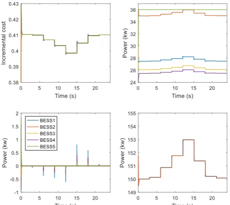
C. Case study 3
In this case, a daily solar power prediction is incorporated to test its robustness under time-varying power generation. The simulation results elaborate the state of BESS and local power state, based on a daily solar radiance curve. Suppose there are 10 houses with solar PV roofs in the microgrid, Fig 5 shows the solar power prediction for each house. Fig 8(a) and Fig 8(b) show the dynamics of the incremental cost and charging power reference provided to BESS in a day. As can be seen from Fig 8, the proposed algorithm has a great potential to overcome weather uncertainty. The power mismatch for each bus converges to zero with the variation of solar power
generation, as shown in Fig 8(c). Fig 8(d) shows total power charged to the BESS in a day.
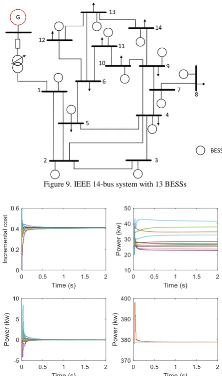
D. Case study 4.
[image:5.595.62.284.257.435.2]In this case, the scalability of the distributed control algorithm is investigated by employing a 14-bus system. The standard IEEE 14-bus system is modified by integrating 13 BESS, as depicted in Fig 9. In the communication network, agent 𝑖 is supposed to exchange the local information with its neighbouring agents. The designed communication graph is strongly connected. The convergence speed can be improved with a higher communication cost, which is accomplished by accommodating more edges between agents. As shown in Fig 10, the proposed algorithm converges within 1 s. The
[image:5.595.311.535.267.449.2]Figure 8. Simulation results of algorithm with solar power supply in a day (a) incremental cost, (b) charging power reference of BESS, (c) supply-demand power mismatch and (d) Total charging power
Figure 6. Simulation results of the distributed algorithm, (a) incremental cost, (b) charging power reference of BESS, (c) supply-demand power
[image:5.595.308.538.504.708.2]power mismatch for each bus converge to zero, as shown in Fig 10(c).
V. CONCLUSIONS
This paper studies statistics models to perform short-term forecasting with solar radiance time-series data. A prescheduled energy dispatch scheme is presented aiming to dynamically regulate power charging of the BESS to alleviate the impact of unstable renewable power generation. The results from three case studies demonstrate the feasibility, robustness and scalability of the control strategy. However, improvements can be made for the next stage work. Firstly, the accuracy of the forecasting model can be improved by taking into account more high-related explanatory variables in the hybrid model. Presently, the proposed algorithm is used for homogeneous BESSs whereas the heterogeneity of various BESSs has not been considered. An advanced algorithm will also be developed to accommodate heterogeneous BESSs.
ACKNOWLEDGEMENT
This research was partially supported by European Regional Development Fund and Entrust Microgrid LLP,
and the Royal Society International Exchanges under Grant IEC\NSFC\170294.
REFERENCES
[1] A. Mellit and A. M. Pavan, “A 24-h forecast of solar irradiance using artificial neural network: Application for performance prediction of a grid-connected PV plant at Trieste, Italy,” Sol. Energy, vol. 84, no. 5, pp. 807–821, 2010.
[2] X. Wu, J. He, Y. Xu, J. Lu, N. Lu, and X. Wang, “Hierarchical Control of Residential HVAC Units for Primary Frequency Regulation,” IEEE Trans. Smart Grid, vol. 9, no. 4, pp. 3844–3856, 2018.
[3] N. Nayak and A. K. Pani, “A Short Term Forecasting of PV Power Generation Using Couple Based Particle Swarm Optimization Pruned Extreme Learning Machine,” Int. J.
Renew. Energy Res., vol. 9, no. 3, 2019.
[4] J. Ma and X. Ma, “A review of forecasting algorithms and energy management strategies for microgrids,” Syst. Sci.
Control Eng., vol. 6, no. 1, pp. 237–248, 2018.
[5] H. M. Diagne et al., “Review of solar irradiance forecasting
methods and a proposition for small-scale insular grids,”
Renew. Sustain. Energy Rev., vol. 27, pp. 65–76, 2013.
[6] S. X. Chen, H. B. Gooi, and M. Q. Wang, “Solar radiation forecast based on fuzzy logic and neural networks,” Renew.
Energy, vol. 60, pp. 195–201, 2013.
[7] J. Liu, W. Fang, X. Zhang, and C. Yang, “An Improved Photovoltaic Power Forecasting Model With the Assistance of Aerosol Index Data,” IEEE Trans. Sustain. Energy, vol. 6, no. 2, pp. 434–442, 2015.
[8] A. Mellit, A. Massi Pavan, and V. Lughi, “Short-term forecasting of power production in a large-scale photovoltaic plant,” Sol. Energy, vol. 105, pp. 401–413, 2014.
[9] G. Delille, B. François, and G. Malarange, “Dynamic frequency control support by energy storage to reduce the impact of wind and solar generation on isolated power system’s inertia,” IEEE Trans. Sustain. Energy, vol. 3, no. 4, pp. 931–939, 2012.
[10] T. Dragičević, X. Lu, J. C. Vasquez, and J. M. Guerrero, “DC microgrids—Part I: A review of control strategies and stabilization techniques,” IEEE Trans. Power Electron., vol. 31, no. 7, pp. 4876–4891, 2016.
[11] M. Longo, W. Yaïci, and F. Foiadelli, “Hybrid Renewable Energy System with Storage for Electrification – Case Study of Remote Northern Community in Canada,” Int. J. Smart Grid, vol. 3, no. 2, 2019.
[12] T. Sakagami, Y. Shimizu, and H. Kitano, “Exchangeable Batteries for Micro EVs and Renewable Energy,” in
Proceeding of 6th Internaional Conference on Renewable
Energy Research and Applications, 2017.
[13] X. Lu, K. Sun, J. M. Guerrero, J. C. Vasquez, and L. Huang, “State-of-charge balance using adaptive droop control for distributed energy storage systems in DC microgrid applications,” IEEE Trans. Ind. Electron., vol. 61, no. 6, pp. 2804–2815, 2014.
[14] N. Kourentzes, F. Petropoulos, and J. R. Trapero, “Improving forecasting by estimating time series structural components across multiple frequencies,” Int. J. Forecast., vol. 30, no. 2, pp. 291–302, 2014.
[15] Y. Xu, W. Zhang, G. Hug, S. Kar, and Z. Li, “Cooperative Control of Distributed Energy Storage Systems in a Microgrid,” IEEE Trans. Smart Grid, vol. 6, no. 1, pp. 238– 248, 2015.
[16] A. J. Wood and B. F. Wollenberg, Power Generation
Operation and Control, 2nd ed. NY,USA: Willey, 1996.
[17] Y. Xu and Z. Li, “Distributed Optimal Resource Management Based on the Consensus Algorithm in a Microgrid,” IEEE Trans. Ind. Electron., vol. 62, no. 4, pp. 2584–2592, 2015.
G
1
2
5 6 12
13
14
11
9
7
3 4
8 10
[image:6.595.57.285.99.485.2]BESS
Figure 9. IEEE 14-bus system with 13 BESSs