Classification Problems with Unequal Error Costs
- Performance of Selected Global Optimization
Algorithms
Andrzej Z. Grzybowski,
Member, IAENG
Abstract—In the paper, an ordinal classification problem with unequal costs of different classification-error-types is considered in the case where the number of classes is greater than 2. It is assumed that each type of classification errors has its specific cost (weight), and the total cost characterizing a given classifier is defined as the expected value of the cost of the classification result. An optimal classifier would be the one that minimizes such a total cost. Thus to find an approximate solution for such a classification problem it is proposed to use Global Optimization (GO) algorithms. The performance of several different types of GO algorithms as tools for solving such a task are compared via computer simulations. The results of simulation experiments are presented and discussed in the paper. Some remarks about the impact of the cost matrix on the probabilities of classification errors related to the developed classifiers are stated as well.
Index Terms—ordinal classification, classification error costs, stochastic search, evolutionary learning.
I. INTRODUCTION
C
LAssification problems consist in identifying the most probable class c an instancev (usually represented by its feature vector x) belongs to. Classification problems are at the core of the field of machine learning (ML). They have been researched intensively over the last decades. In litera-ture, one can find great many different classifiers developed under different assumptions about the classification problems as well as by the adoption of different learning algorithms, e.g. [5], [2]. However, after studying many classification problems of different types and of various underlying nature, it is clear to the machine-learning community that there is no single classification algorithm that is superior with all respects and for all datasets [9], a conclusion analogous to famous no free lunches theorem in the theory of stochastic search and optimization [7]. On the other hand, it appears that some learning algorithms outperform others for some specific problems and/or types of data.In this paper we focus on the ordinal classification prob-lems, i.e. problems where the class label (target variable) takes on values in a set C={c1, . . . , ck} of categories that exhibit a natural ordering. We consider multiclass problems, it is the case where the number k of classes is greater than 2. Then we havek(k−1)different classification errors with, possibly, different consequences. Thus we assume that to each of these errors it is assigned its specific error-cost (weight) that represents the importance of its negative repercussions. An index of performance of a classifier is defined as the expected value of the classification-result-cost,
Manuscript received June 19, 2019; revised July 16, 2019.
A.Z. Grzybowski is with the Institue of Mathematics, Faculty of Mechani-cal Engineering and Computer Science, Czestochowa University of Technol-ogy, Czestochowa, 42-201 Poland, e-mail: [email protected]
and the optimal classifier is the one that minimizes this index. Consequently, the learning algorithms are aimed at finding a classifier that minimizes such an index on the training set. However, due to the fact that the optimality criterion cannot be expressed by any closed-form-mathematical expression and the value of the criterion can only be evaluated for each specific classifier separately, the minimization problem cannot be solved directly. What is more, it implies that when looking for the expected cost minimum we have to confine ourselves to gradient-free optimization methods. Thus in presented studies global optimization (GO) methods that are based on the idea of the stochastic search are proposed to cope with such a task. These methods require only few assumptions about the underlying objective functions -they have the so-called ”black box” character, see [7], [8]. Evolutionary techniques have been employed to solve various specific classification problems and related tasks, [12], [2], [5]. In this paper we use computer simulations to study the performance of some popular stochastic global optimization methods as learning tools for some specific type of ordinal classification problems. We focus here on the following GO techniques: the genetic algorithms, evolutionary search with soft selection and simulated annealing. Some remarks about the impact of the error-cost-matrix on the probabilities of a particular error occurrence are formulated as well.
The paper is organized as follows. In Section 2 the specific type of classification problems considered in this paper is introduced formally. Section 3 provides us with the description of considered gradient-free GO algorithms. The simulation framework for our experiments as well as the simulation results with discussion are presented in Section 4. The paper is concluded with final remarks and comments.
II. PROBLEMFORMULATION
belongs to class Ci given its score value s. In considered multiclass case with assumed above ordering relation onC, the values of any reasonable scoring classifiers need to satisfy the following monotonicitycondition (MC):
If
i < j andP(Ci|s1=f(x1))< P(Cj|s1=f(x1)) then
P(Ci|s2=f(x2))< P(Cj|s2=f(x2)) for anyx2 such thats1< s2. :
Such a scoring classifierf can be used with a given vector of thresholds (t0 =−∞, t1, . . . , tk−1, tk =∞) to produce a discrete classifierg:
g(x) =Ci if and only if ti−1< f(x)≤ti (1)
It is obvious that in real-world problems the misclassifi-cation errors are unavoidable. It is also well understood that there are many problems where various kinds of classification errors have consequences of significantly different impor-tance. It can be observed in such areas as medical diagnosis, finance/banking security, in classification of construction elements according their structural properties etc. In all such cases these differences should be reflected in the overall cost of classification process. Letdij,i, j= 1, . . . , k, denote the situation (an event) where an instance represented by the feature vector xis classified asci while its true class iscj. Obviously the eventsdii represent the correct classifications, while dij, i6=j, represent classification errors. Let us also consider a matrix W = [wij], the elements of which repre-sent the weights that reflect the importance of related events dij. Let additionally P r = [pij] denote a matrix with the elementspij being the probabilities of eventsdij. Obviously these probabilities depend on the adopted classifier g. Thus the total cost of any classifiergis given here by the following formula:
T C(g) =X
i6=j
pijwij− X
i
piiwii (2)
The total cost given by (2) consists of two parts. The first sum reflects the expected loss related to misclassification errors, whilst the second one represent the expected bene-fits that result from the correct classification. The optimal classifier would be the one that minimizes this total cost. Obviously such a classifier cannot be found without precise knowledge about the matrix Pr. However to obtain an ap-proximate solution, for any given classifier we can estimate this matrix on the basis of the training set T S. The process of finding the minimum of the functional (2) based on the training set T S is called classifier learning process, and the algorithms used for this purpose are frequently called the learning algorithms.
In our study we confine ourselves to discrete classifiersg that are based on the scoring linear classifiers, i.e.f(x, α) =
x.αT,∈Rn. Consequently, our aim is to find vectorsα∈Rn andt∈Rk−1 such that classifierg given by (1) minimizes the functional (2) estimated on the basis of the given training setT S. For simplicity, any of these classifiersgwill be iden-tified with the corresponding vector z= (α,t)∈Rn+k−1. As candidates for the learning algorithms we consider GO ones described in the next section.
III. GRADIENT-FREE GLOBAL OPTIMIZATION ALGORITHMS
Evolutionary methods (EM) are perhaps the most popular search methods used for the global optimization tasks. All EM algorithms are computer-based approximate representa-tions of natural evolution. In these types of algorithms the population (of potential solutions) is changed/transformed during a sequence of generations according to stochastic analogues of the natural processes of evolution. The EM algorithms are divided into two main groups: genetic algo-rithms and evolutionary programming methods, [7]. Genetic algorithms (GAs) are a subclass of evolutionary algorithms where the elements of the search space are binary strings in this theory called genotypes or chromosomes. The genotypes are used in the reproduction operations while the values of the objective functions (so-called fitness) are computed on basis of the phenotypes in the original problem space which are achieved by the genotype-phenotype mapping. The version of this algorithm implemented in our learning process can be described as follows, [3]:
Letz= (α, t)∈Rn+k−1
•
Step 0 (Initialization) Set the initial parent population of K vectors zi∈Rn+k−1, i= 1,2, . . . , K.
Step 1 Assign to each vector zi, i= 1, . . . , K, its fitness i.e. the value of the criterion F(zi).
Step 2 Select with replacement K parents from the full population. The parents are selected with probabil-ity proportional to the their fitness.
Step 3 For each pair of parents identified in Step 2, per-form crossover on the parents chromosomes at a randomly (uniformly) chosen splice point.
Step 4 Replace all K parent-chromosomes of current parent-population with the chromosomes of current offspring-population from Step 3. Then mutate the individual bits with uniform probability.
Step 5 Compute the fitness values for the population of N phenotypes corresponding to new chromosomes. Terminate the algorithm if the stopping criterion is met; else return to Step 2.
Step 6 Return the so far best generation and the fitness of its elements
In difference to the GAs, the evolutionary programming methods (EP) operate directly with the floating-point repre-sentations. In evolutionary programming, a solution candi-date is thought of as a phenotype (specimen) itself. Thus, selection and mutation are the only operators used in EP and recombination (crossover) is usually not applied. There are various implementations of this idea in literature. In our simulations the performance of the so-called algorithm of the evolutionary search with soft selection (ES ) was examined. The algorithm implemented in our simulations is the following:
•
Step 0 (Initialization) Set the initial parent population of K vectors zi∈Rn+k−1, i= 1,2, , K.
Step 1 Assign to each vector zi, i= 1, , K, its fitness i.e. the value of the criterionF(zi).
Step 2 Select a parentv by soft selection i.e. with proba-bility proportional to the its fitness.
Step 3 Create a descendant w from the chosen parent v
is a randomn-dimensional vector with coefficients having expected value equal to zero and given standard deviation.
Step 4 Repeat steps 2 and 3 for K times to create a new K-element generation of n-dimensional vectors (so-called descendants)
Step 5 Replace the parent population with the descendant population
Step 6 Repeat the 1 to 5 steps until the stopping criterion is met
Step 7 Return the so far best generation and the fitness of its elements
In our study any specimen from the current population (generation) is selected as a parent (Step 2) with probability proportional to its relative fitnessRF given by the formula:
RF(x) = 90F(x)−Fmin
Fmax−Fmin
+ 10
If theFmax=Fmin,than these probabilities are the same for each elements of the population.
The third method adopted in our studies is the Simulated Annealing Algorithm (SA). It is perhaps historically first global optimization method based on stochastic search idea. It was developed by Kirkpatrick in the early 1980s although the main idea was introduced by Metropolis in 1953, [7]. In difference to the previously described EMs, this class of algorithms does not use any biology-inspired mechanisms. Instead, the underlying idea is adapted from material science. Annealing is a heat treatment of material with the goal of altering its properties such as hardness. Metal crystals usually have some small defects which weaken its overall structure. By heating the metal, the energy of its ions and, thus, their diffusion rate is increased. Then, their dislocations can be destroyed and the structure of the crystal is reformed as the material cools down and approaches its equilibrium state. When annealing metal, the initial temperature must not be too low and the cooling must be done sufficiently slowly so as to avoid the system getting stuck in a meta-stable, non-crystalline, state representing a local minimum of energy.
For the global optimization purpose the idea can be implemented in various ways. The algorithm implemented in our studies is as follows, see e.g. [7], [3]:
•
Step 0 (Initialization) Set an initial temperature T and initial solution z =zcurr; determine the criterion valueF C =F(zcurr)
Step 1 Relative to the current value zcurr, randomly de-termine a new value of znewRn, and compute F N=F(znew)
Step 2 Let d=F N −F C. Ifd < 0 accept znew;, else, accept znew only if a random variable U having the uniform p.d. on the interval [0,1] satisfies U < exp[−d/T]. If znew is accepted then zcurr is replaced byznew; elsezcurr remains as is. Step 3 Repeat steps 1 and 2 for given numberKT times. Step 4 LowerT according to the annealing schedule and return to Step 1. Continue the process until the stopping criterion is met.
Step 5 Return the best solutionzbfound during the
cool-ing process and the valueF(zb)
During the simulation process the initial ”temperature” T decays geometrically in the number of ”cooling phases”.
Specifically, in our simulations the new temperature is related to the old temperature according toTnew= 0.7Told. Another area for different implementations is in step 1, whereznewis generated randomly. In this study it was generated according the formula znew = zcurr +U, where U is a random n-dimensional vector with coefficients having expected value equal to zero and given standard deviation s, the latter starts with value 0.4 and decays during the simulation process similarly as the temperature.
It is worth noticing here that the simulated annealing algorithm is designed for minimization tasks, while the previ-ous two methods are designed directly for the maximization ones. Thus the fitness function used in our implementation of the GA and ES is defined as F(g) = A−T C(g) . In the SA, the fitness F is given by the opposite values. To make all the results comparable, the SA returns −F(g)
as the best fitness value found by the SA algorithm, see the step 5 in its description. In our experiments constant A=1 to assure positivity od F. For any given problem it is likely that the performance of one algorithm will be superior to others. However, it is rarely possible to know a priori which algorithm is superior. FamousNo Free Lunch theorems state that when averaging over all optimization problems all search algorithms work the same (i.e., none can work better than a blind random search),[7]. This remark also concerns the learning algorithms, see [9]. On the other hand the NFL theorems do not address the performance of a specific algorithm applied to a specific class of criterion functions. They compare the performance of algorithms over all problems, where each problem can be considered equally likely. It is well known however, that for some specific types of problems some algorithms may perform extremely well, while other perform very poorly. Indeed, some literature reports that evolutionary techniques has been successfully applied in various classification tasks and related more specific problems, [2], [12], [11], [1], [10], [13].
One of our goals here is to determine which of the above introduced algorithms (if any) is superior in learning the classifiers (1) under the criterion given by (2).
IV. SIMULATION FRAMEWORK AND RESULTS
and the classes exhibit the required natural ordering. The set of vectors (xi, ci) ∈ Rn+k−1, i = 1, , N, forms (random) training set T S for our simulation experiment.
For any generated T S we use the learning algorithms described in Section 3. The results we are interested in are
- the approximated minimal costsT Cassociated with the best classifier learned by a given learning algorithm and - the corresponding ”best” matrixP r.
The former is used for direct comparisons of the best classifiers found by adopted learning approaches, while the latter contains detailed information about the probabilities of successful classifications as well as the probabilities of any specific classification errors.
It is well known that these results depend on the specific implementation of the GO algorithms, especially on the number of elements in populations and on the assumed number of the subsequent generations. Thus, to assure some kind of objectivity of the comparisons, in our experiments the total number of calculations of the fitness-function-values is fixed, and for each of these algorithms it equals 300000. For each fixed numbers k and n the performance of the algorithms are compared under various types of the weight matricesW. All these matrices are normalized to 1, then for each of them the experiments are repeated for 30 different TS and next the results are averaged. In every experiment the initial population (or initial element in the SA algorithm) is assumed as the set of classical discreetregressionclassifiers (RC), so each element in the initial population is the same. The regression classifiers are also used as the reference classifiers in our studies, i.e. we compare their character-istics (such as the total cost or probabilities of successful classification) with the ones related to the considered GO classifiers. Table I summarizes the results.
It can be seen that the GA outperforms all other considered algorithms - its total cost is the least one in every studied case. Moreover, although it was not the main purpose of the learning, the probabilities of correct classification (PrS) are the highest ones and they are very close to 1 in the examined cases. The symbol RI stands for therelative improvementof the latter characteristic (with respect to the RC) and its value is presented in the last column of the table.
Now let us turn our attention to the issue of the dependence between the weight matrices and the resulting matrices of probabilities P r of the correct/incorrect classifications. As we know in general the elements on the principal diagonal in P r, as being the probabilities of correct classification, should be close to 1, and all the remaining ones should be close to 0, as probabilities of misclassification. However, if the misclassification errors have different costs than it is important, that these errors which are - say - more dangerous would actually occur with smaller probabilities than others. It should be achieved by proper choice of the weight matrix
W. In order to verify whether or not the elements of the weight matrix Wdo really impact the resulting probability matrix P r, a number of different weight matrices W were assumed in the experiments. Let us look a little bit closer into several interesting examples.
[image:4.595.312.539.529.697.2]So, first let us consider case where the number of classes isk= 4and the weight matrix W1is the following.
TABLE I: Average results simulated under various asymmet-ric weight matasymmet-rices W. Considered GO learners are the GA, ES and SA, as defined in Section 2. A reference classifier is the regression one, it is labelled as RC. The BS stands for the random blind search
Learning algorithm F PrS RI k=3,
RC 1.31 0.82
-ES 1.33 0.84 2.0%
GA 1.41 0.97 18.8%
SA 1.33 0.72 -12%
BS 1.28 0.75 - 15%
k=4
RC 1.18 0.73
-ES 1.20 0.77 5.0%
GA 1.26 0.94 30.2%
SA 1.19 0.73 0.1%
BS 1.15 0.64 - 12%
k=5,
RC 1.09 0.61
-ES 1.12 0.67 10.2%
GA 1.17 0.87 42.0%
SA 1.12 0.67 10%
BS 1.09 0.56 - 9%
W1= 1 14
1 0.9 1.8 2.7 0.1 1 0.9 1.8 0.2 0.1 1 0.9 0.3 0.2 0.1 1
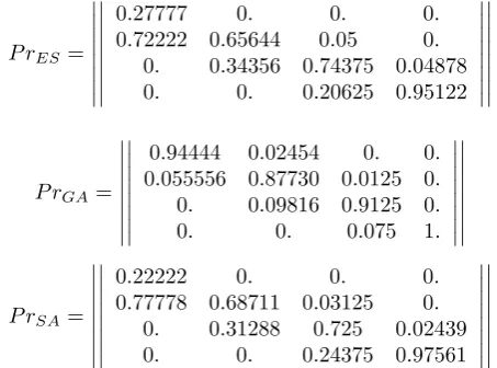
The above matrix is normalized to 1 ( we use the normalizing constant 1/14). We present it in such a form to make it easier to note that the weights related to the errorsdij , see Section II, are the greater, the greater is the value of j−i. So, it reflects the case where the classification of a given instance to the class that is higher than the one it actually belongs to is more costly (dangerous) than the erroneous classification to a lower class. Now let us look at the matricesP r related to best classifiers learned by the considered GO algorithms (these algorithms are indicated in the subscript of the matrix symbol) .
P rES=
0.27777 0. 0. 0.
0.72222 0.65644 0.05 0.
0. 0.34356 0.74375 0.04878 0. 0. 0.20625 0.95122
P rGA=
0.94444 0.02454 0. 0.
0.055556 0.87730 0.0125 0.
0. 0.09816 0.9125 0.
0. 0. 0.075 1.
P rSA=
0.22222 0. 0. 0.
0.77778 0.68711 0.03125 0.
0. 0.31288 0.725 0.02439 0. 0. 0.24375 0.97561
Similar in spirit results we obtain in the case where the weight matrix is the transposition of the above one - obvi-ously, this time the probabilities of erroneous classifications to higher classes are the greater ones. To save the article space we omit here the presentation of the corresponding matrices P r related to best classifiers obtained by our learning algorithms.
Our last example concerns the importance of weights assigned to correct classifications, i.e. the role of the diagonal elements wii, i = 1, . . . , k in the matrix W. It is not obvious, whether the ”rewards” for correct classification -reflected by positive values ofwii, i= 1, . . . , k- are impor-tant for the proper-classifier-learning. Or maybe solely the ”punishment” for incorrect classification would be enough for the classifier-learning tasks. To answer these questions let us consider a weight matrix similar to the above-presented
W1, but with 0s on the principal diagonal, i.e. our weight matrix is now the following:
W0= 1 10
0 0.9 1.8 2.7 0.1 0 0.9 1.8 0.2 0.1 0 0.9 0.3 0.2 0.1 0
Now the related matricesP r look as follows.
P rES=
0.45 0. 0. 0.
0.55 0.54369 0. 0.
0. 0.45631 0.77143 0.
0. 0. 0.22857 1.
P rGA =
1. 0. 0. 0.
0. 0.980583 0.0047619 0.
0. 0.0194175 0.957143 0.
0. 0. 0.0380952 1.
P rSA=
0.5 0. 0. 0.
0.5 0.61165 0.00952 0.
0. 0.37864 0.73810 0.
0. 0.00971 0.25238 1.
We see that the diagonal elements of the weight matrix play an important role in the learning tasks. All considered learning algorithms produce much worse classifiers in the cases with a lack of reward for proper classification - solely the punishment for misclassification is not enough. However, it is again worth emphasizing, that the GA algorithm outper-forms the other two also in such cases.
V. FINAL REMARKS AND CONCLUSIONS
Based on the presented simulation results one can con-clude that among considered GO algorithms, the GA is the best one as a tool for classifier-learning tasks in the ordinal classification problems. This observation is also confirmed by our simulations conducted for greater numbers of classes than those presented in Table I. The GA algorithm performs really well - the average probability of correct classification of an instance is about 0.9 and one hardly can expect higher frequency of correct decisions in such uncertain decision problems. Our simulations show that these probabilities of success decrease when the number of classes increases - a fact that is rather intuitive. However, it is worth noticing that, in spite of this perhaps natural tendency, the supremacy
of the GA over the remaining learning algorithms increases when the number of classes increases, see the last column in Table I. However, one should be aware that in problems with unequal costs of classification errors, the probabilities of correct classification are not necessarily the most crucial ones. It is worth emphasizing that, instead, sometimes it is even more important not to makespecificclassification errors (in a given specific problem). In such cases one should focus on the weight matrix - proper construction of the matrix is of primary interest in all classification problems with unequal costs of misclassification errors. Our simulation experiments revealed some important facts about the influence of the weight matrix on the classifier-learning results.
The examples presented in Section IV, as well as many other results that we have obtained during our simulations, confirm that the proportions between the weights of par-ticular classification errors have a proper impact on the proportions between corresponding probabilities of errors and, again, the GA learning algorithm is the best with respect to this issue. Moreover, it was also shown, that the weights assigned to correct classifications are also very important, they make it easier for the learning algorithm to lower the probabilities of misclassification. Thus, the role of both the reward and punishment revealed by our results concerning machine learning is in line with the operant-conditioning principle formulated by Skinner to explain human-learning nature, [4] .
REFERENCES
[1] Choo Jun Tan, Ting Yee Lim, Chin Wei Bong, Teik Kooi Liew, (2017) ”A multi-objective evolutionary algorithm-based soft computing model for educational data mining: A distance learning experience”, Asian Association of Open Universities Journal, Vol. 12 Issue: 1, pp.106-123, [2] Espejo,P.G., Ventura, S., Herrera, F., (2010) ”A Survey on the Appli-cation of Genetic Programming to ClassifiAppli-cation”, IEEE Transactions On Systems, Man, And Cybernetics-Part C: Applications And Reviews, Vol. 40, No. 2, 121-144
[3] Grzybowski, A.Z. (2011) ”Simulation analysis of global optimization algorithms as tools for solving chance constrained programming prob-lems”, Acta Eletrotechnica et Informatica, Vol 11 (4), 60-65 [4] McLeod, S. A. (2018). ”Skinner - operant conditioning.”, Retrieved
from https://www.simplypsychology.org/operant-conditioning.html (ac-cessed 14.06.2019)
[5] Mane S., Sonawani, S. S. , Sakhare S., and Kulkarni, P. V., (2014), ”Multi-objective Evolutionary Algorithms for Classification: A Re-view”, International Journal of Application or Innovation in Engineering and Management, 292-297
[6] Obuchowicz, A., Korbicz, J.: ”Global optimization via evolutionary search with soft selection”, unpublished manuscript, available: http://www.mat.univie.ac.at/∼neum/glopt/mss/gloptpapers.html (accessed 14.06.2019)
[7] Spall, J.C.: Introduction To Stochastic Search And Optimization; Esti-mation, Simulation, And Control , John Wiley and Sons. Inc., Publica-tion, 2003.
[8] Weise, T.: Global Optimization Algorithms - Theory and Applica-tion,ebook available at http://www.it-weise.de/projects/book.pdf (ac-cessed 14.06.2019)
[9] Wolpert, D.H. (1996), ”The lack of a priori distinctions between learning algorithms.”, Neural computation 8(7), 1341-1390
[10] Zhang, M., Smart, W. (2004) ”Multiclass object classification using genetic programming”. Applications of Evolutionary Computing, pp. 369-378.
[11] Zhang, M., and Wong, P. (2008) ”Genetic programming for medical classification: a program simplification approach.” Genetic Program-ming and Evolvable Machines 9, 229-255.
[12] Xue, B., Zhang, M., Browne, W. N., And Yao, X. (2016) ”A survey on evolutionary computation approaches to feature selection.”, IEEE Transactions on Evolutionary Computation 20, 606-626.